Alternating Graves’ Hyperthyroidism and Hashimoto’s Hypothyroidism for more than 20 Years: A Case Report - Juniper Publishers

 Endocrinology and Thyroid Research - Juniper Publishers

Abstract

Background: Graves’ disease (GD) and Hashimoto thyroiditis (HT) are autoimmune thyroid diseases. Around 20% of patients with GD develop spontaneously Hashimoto hypothyroid, contrarily, with less frequency occurred that a patient with HT became hyperthyroid during its clinical course. In the present case, a patient shows spontaneous oscillations of her thyroid function over a period of 21 years.

Case report: A 78-year-old woman presented GD, her medical history was notable for had been diagnosed with GD at 58-year-old, she was treated for 18 months with antithyroid drug (ATD). After withdrawal of ATD, she remained in remission for 9 years. Later, she developed HT with frank hypothyroidism, and was treated with levothyroxine for 12 years. At the end of this period, she had Graves’ hyperthyroidism again and was treated with Metimazole for 14 months before returning to hypothyroidism.

Conclusion: there are very rare cases that have an oscillating course, alternating GD, and HT for decades, whose pathogenesis is pending clarification. This case supports the view that GD and HT are two ends of the same spectrum.

Keywords: Graves’ disease 1; Hashimoto thyroiditis 2; autoimmune thyroid disease 3.

Abbreviations: AITD: Autoimmune thyroid diseases; HT: Hashimoto’s thyroiditis; GD: Graves’ disease

Introduction

Autoimmune thyroid diseases (AITD) are organ-specific autoimmune diseases. AITD are the most prevalent alterations that affect the thyroid gland. AITD comprises interrelates conditions: Hashimoto’s thyroiditis (HT), Graves’ disease (GD), atrophic autoimmune hypothyroidism, postpartum thyroiditis, the first two being the most prevalent. The common pathological feature of AITD is the presence of lymphocytic, mainly T cells infiltrate the thyroid gland that may progressively replace the thyroid tissue. Variable thyroid follicular cell atrophy and fibrosis are characteristic of HT, while in GD thyroid follicles are hypertrophied. Anti-tiroperoxidase antibodies (TPOAb) are a sensitive marker of ATID both in HT and GD. Thyroid stimulating hormone receptor antibodies (TSHR-Ab) are characteristic of GD and responsible for hyperthyroidism [1]. One form of AITD may change to another as the course of the immune process progresses [1]. Around 12 % - 20% of patients with GD spontaneously develop Hashimoto hypothyroid after antithyroid drug (ATD) discontinuation [2-4]. Contrarily, with less frequency occurred that a patient with HT became hyperthyroid during its clinical course [5]. In the present case, a patient shows spontaneous oscillations of her thyroid function over a period of 21 years.

Case Presentation

A 78-year-old woman, with anxiety begins to be noticed from about 6 months. Three months later, she added to her symptomatology palpitations, dyspnea and edema in the lower extremities that increase in intensity slowly. Then she requests medical attention in an endocrinology consultation. She was diagnosed with hypothyroidism 12 years ago and treated with 75 mcg/day of levothyroxine. She had not done control thyroid tests for 2 years due to the covid-19 pandemic. A month before the Endocrine consultation, she was attended in a primary care center, for worsening of dyspnea, palpitations, and increased edema in the lower extremities and tachyarrhythmia. Thyroid function tests were done, showed elevation of free T4 and decrease in TSH levels, doctor recommended reducing the dose of levothyroxine to 25 mcg /day, added diuretic (Furosamide) and beta-adrenergic blocker (Bisoprolol) drug to her treatment. Two weeks later due to worsening of her symptoms, she came to our Endocrine office.

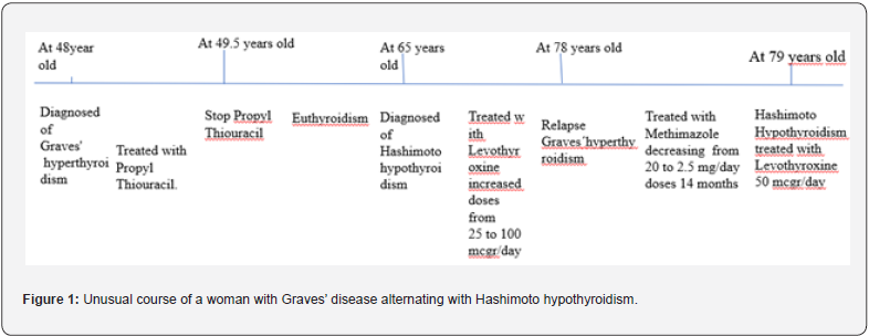
Personal medical history was notable for having been diagnosed with Graves’ hyperthyroidism at 58-years-old when living in Houston (USA), she was treated for 18 months with ATD (Propyl-thiouracil). After withdrawal of ATD, she remained in remission for 9 years. Later, she developed Hashimoto’ thyroiditis with frank hypothyroidism, treated with increasing doses of levothyroxine for 12 years. Physical examination revealed a female patient 1.60 meters tall, and 59 kg weight. Blood pressure 150/100, the patient had frank dyspnea, with a fibrillar tremor in both hands, pulse 100/min, with frequent extrasystoles. She also had edema in both ankles. She was diagnosed with relapse of Graves’ hyperthyroidism, and prescribed as treatment: rest, suppress levothyroxine, and administration of Methylmazole (MMI) of 5 mg, 4 tablets per day, and Bisoprolol 2.5 mg every 12 hours. It is also recommended to quit smoking.

Six weeks later, the patients felt better, presented light dyspnea, rhythmic pulse at 76 beats per minute, no edema. The thyroid function test showed Free T4, Free T3, and TSH within the reference values (Table 1). MMI doses were reduced to 2 tablets per day. Two months later she was asymptomatic with thyroid function test within reference values. MMI dose was reduced to 1 tablet per day. Eight weeks later, in view of the results of the thyroid function tests, MMI were reduced to 1 tablet 5 days and a half tablet 2 days. Two weeks after she became to fill anxiety and palpitations, a new function test performed 4 weeks later, revealed a slight increase of Free T4 and Free T3, Table 1, and then MMI dose was increased to 1 tablet per day. The symptoms disappear 10 days later. MMI was maintained until the levels of anti-TSH receptor antibodies were negative. Fourteen months after the diagnosis of GD recurrence, and two months after MMI withdrawal she again presented hypothyroidism demanding treatment with levothyroxine (Figure 1).

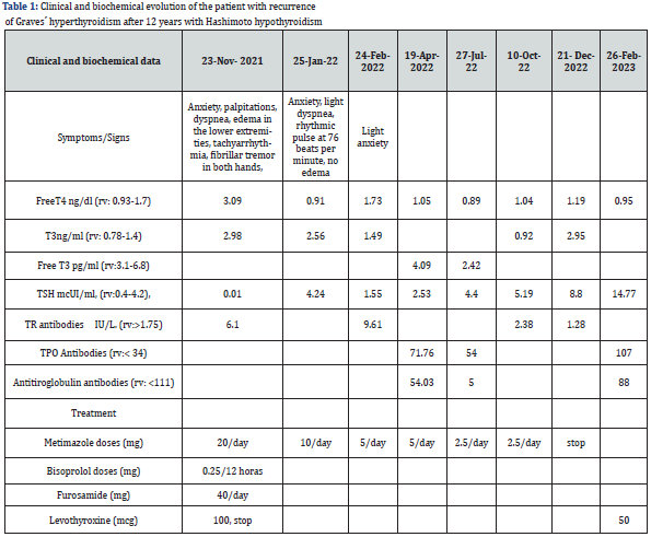
The hormone tests performed included determinations of serum Free T4 (FT4) (reference values: 0.93-1.71 ng/dl), Free T3 (FT3) (reference values: 2.55-4.33 pg/ml), Thyrotropin hormone (TSH) (reference values: 0.30-4.50 mUI/L), all of which were analyzed by an immunochemiluminescent assay, IMMULITE (Diagnostic Products Corp. Los Angeles, CA, USA). The levels of both Thyroid peroxidase antibodies (TPOAb) and thyroglobulin antibodies (TgAb) were measured by a chemiluminiscent assay (Immulite 2000, Diagnostic product Corp, Los Angeles, CA, USA, with reference values of 0-30 and 0-40 mIU/ml respectively. The concentration of Thyroid receptor antibodies (TRAb) (reference values 0-10 IU/L) was measured using a radioreceptor assay (TRAK-assay; Henning, Berlin, Germany). The intra-assay and inter-assay CVs were 5% and 7.5% respectively. South Galicia is an area with sufficient iodine intake [6]. Long-term remission was defined as the absence of clinical manifestations of hyperthyroidism, together with biochemical euthyroidism and negative TRAb values, at least 12 months following the withdrawal of ATDs [7].

Discussion

Autoimmune thyroid disease results from dysregulation of the immune system leading to an immune attack of the thyroid gland. The AITD comprise two main clinical presentations: HT and GD. The clinical hallmark of these conditions is hypothyroidism and hyperthyroidism, respectively. One form of clinical presentation can change to another as the immunological process progresses. There have been cases of patients switching from Graves’ hyperthyroidism to Hashimoto hypothyroidism, being less frequent patients switching from hypothyroidism to hyperthyroidism [8], due to the critical loss of thyroid mass that can respond with TSHR Ab [9], although it is described some patient who developed frank hyperthyroidism and required treatment with ATD [10]. The shift from Graves’ disease to Hashimoto’s disease and vice versa in the same patient suggests that both would be the same disease that can be expressed in two ways. However, genetic studies indicate that GD and HT are modestly related diseases [11].

In the present case report, a woman initially diagnosed with Graves’ hyperthyroidism treated with ATD for two years. After withdrawal of ATD she remained in remission for 9 years. After which she developed Hashimoto’s thyroiditis, being treated with increasing doses of levothyroxine. Twelve years later, frank Graves’ hyperthyroidism requires treatment with ATD. She was treated with MMI for 14 months. Finally, after two months of withdrawal ATD she developed Hashimoto’s hypothyroidism needing small doses of levothyroxine. Cases of alternating hyperthyroidism and hypothyroidism are very rare [12]. The unusual course of this case supports the view that it is the same disease that can be expressed from both hyper- and hypothyroidism.

Some authors postulated that the pathogenesis of patients alternating hyperthyroidism and hypothyroidism is due to the balance between the levels of stimulating TSHR-Ab with thyroid Blocking hormone receptor antibodies (TBHR-Ab) [13]. However, in patients with long-term course, when presented HT, follicular cells are destroyed to a variable extent, depending on the chronicity of the HT related hypothyroidism [14], and for the development of frank hyperthyroidism requires a restoration, at least partially, of the mass of follicular cells of the thyroid. Thus, the pathogenesis of such a phenomenon is pending clarification.

This case also draws attention to the fact that we must bear in mind that patients with long-standing autoimmune hypothyroidism can be transformed into frank hyperthyroid ism, which requires diagnosis and treatment without delay. Some authors believe that given the unpredictability of the diseases in these patients who alternate hyperthyroidism and hypothyroidism, ablative treatment would be advised [10]. In my opinion, educating patients and their families about the nature of the disease, its clinical characteristics, and an annual follow-up, can be sufficient to manage these cases properly, avoiding postablative hypothyroidism that is not easy to handle, in addition, if we avoid ablative treatment, we can know the natural history of Graves’ disease in more patients, without any added risk [15].

Conclusion

Although very rare, there are cases of patients who spontaneously alternate long-term periods of Graves’ hyperthyroidism with Hashimoto related hypothyroidism for decades, whose pathogenesis is pending of clarification. The present case supports the view that GD and HT are two ends of the same spectrum. Clinicians must also keep in mind that although rare, these cases exist and require diagnosis and treatment without delay.

To Know more about Journal of Endocrinology and Thyroid Research

Click here: https://juniperpublishers.com/jetr/index.php

To Know more about our Juniper Publishers

Click here: https://juniperpublishers.com/index.php

A Review on Some Important Notes about the Surgical Anatomy of the Internal Jugular Vein - Juniper Publishers

 Anatomy Physiology & Biochemistry - Juniper Publishers

Abstract

Internal Jugular Vein is an important anatomical structure in the head and neck region. As a paired jugular vein, it originates from sigmoid and inferior petrosal sinuses. At the skull base level, it begins at the jugular foramen posterior compartment. Then it goes down to the neck. It collects blood from some parts of the face and neck and also the brain.

Considering the importance of having knowledge about the anatomy of the internal jugular vein specifically for the surgeons and other clinicians who are dealing with the patients with head and neck and vascular pathologies, this brief review tries to point to some important anatomical aspects related to the internal jugular vein as well as some important clinical points.

Keywords: Jugular Vein; Internal; Anatomy; Surgery; Clinical Relevance

Body

Internal jugular vein as a paired jugular vein, originates from sigmoid and inferior petrosal sinuses and is usually known as the largest neck vein. At the level of the skull base, it begins at the jugular foramen posterior compartment and since it is somehow dilated at its original part, it would be named as superior bulb at this level. Internal jugular vein runs downward in an almost vertical direction in the carotid sheath.

Internal jugular vein has some relations with the internal carotid artery at different levels. At the C2 level, internal jugular vein would be in the posterior part of the internal carotid artery. Then it turns towards the lateral direction while still being in the posterior part of the artery which at the level of C3, internal jugular vein would be in a posterolateral part of the internal carotid artery. At the level of C4, the internal jugular vein would be located at the lateral part of the internal carotid artery. It is important to notice that the tenth cranial nerve lies between the internal jugular vein and the internal carotid artery. After leaving the carotid sheath, deep cervical lymph nodes surround the internal jugular vein. In a downward direction, the internal jugular vein lies on the lateral mass of the first cervical vertebra, prevertebral fascia, middle scalene muscle, anterior scalene muscle and the cervical pleura dome.

In case of dividing the internal jugular vein into three anatomical parts meaning upper, middle, and lower thirds, it will be crossed and overlaid by different anatomical structures. The eleventh cranial nerve’s spinal root would cross the internal jugu lar vein at its origin. The middle third of the internal jugular vein would be crossed by the inferior root of the ansa cervicalis. The lower third of the internal jugular vein would be covered by the omohyoid muscle tendon and the sternocleidomastoid muscle. Usually, the right internal jugular vein is larger than the left one because its blood drainage is done from the superior sagittal sinus which in contrast with the left one meaning the inferior sagittal sinus, is larger in its size [1-4].

From the clinical point of view and at the bedside, the internal jugular vein can be found while it runs from the posterior part of the jaw angle to the posterior part of the sternoclavicular joint. Central venous catheterization with or without the ultrasound guidance, would preferably be done through the internal jugular vein. Estimation of the jugular venous and right atrium pressures and also estimation of the patients hemodynamic status, can be done at the bedside by observing the internal jugular vein. In Trauma settings, the internal jugular vein is susceptible to various damages given its superficial course in the neck. So, any blunt or penetrating trauma can cause injury to the internal jugular vein which result in the occurrence of hemorrhage and increased risk for the occurrence of air embolism. Thrombosis of the internal jugular vein and Lemierre syndrome which is known as a thrombosis of the internal jugular vein due to infection of the pharynx, are another pathologies which can affect the internal jugular vein.

Surgery of the internal jugular vein requires paying enough attention to its and surrounding anatomical structures. Surgical repairing of the internal jugular vein should be considered first and during this, it should be tried by the surgeon to limit the amount of narrowing the vessel as much as possible. Ligation may be necessary in the cases which the amount of damage to the vessel is high.

In any of these cases, care should be taken to avoid causing injury to the surrounding anatomical structures like internal carotid artery and the tenth cranial nerve. In case the carotid sheath is affected by the injury, the surrounding anatomical structures should be evaluated for possible injury and necessary surgical repair as well [2,5,6].

Conclusion

Internal jugular vein is an important anatomical structure which having detailed knowledge about its anatomy is of great importance specifically for the surgeons and other clinicians whom are dealing with the patients with head and neck and vascular pathologies, to approach its relevant pathologies and damages with more precision and with lowest surgical complications at the bedside.

To Know more about Anatomy Physiology & Biochemistry International Journal

Click here: https://juniperpublishers.com/apbij/index.php

To Know more about our Juniper Publishers

Click here: https://juniperpublishers.com/index.php

Response Surface Methodology-A Statistical Tool for the Optimization of Responses - Juniper Publishers

 Addiction & Rehabilitation Medicine - Juniper Publishers

Abstract

Experimentation plays a significant role in Science and Technology, which is an application of handling experimental units, and then the determination of one or more responses from that. In every experiment, some inputs (x) transform into results that have one or more observable response variables (y). Therefore, from the results, the conclusion can be drawn by experiment. For obtaining an unbiased conclusion a researcher needs to plan & design the experiment and analyze the results obtained. When dealing with a continuous range of values then the true connection between y and x’s might not be known. In such cases, statistical analysis like Response Surface Methodology plays a crucial role, which is a combination of statistical and mathematical techniques useful for designing and analyzing problems where a response of interest is affected by several variables, and the objective is to optimize this response. It generally helps in reviewing the empirical relationship among one or more measured responses and various independent variables in the form of a polynomial equation. Mapping of those responses associated with the experimental domain helps in generating an optimized method.

Introduction

Response Surface Methodology [1-9] (RSM) plays a crucial role, which is a combination of statistical and mathematical techniques useful for designing and analyzing problems where a response of interest is affected by several variables, and the objective is to optimize this response. It generally helps in reviewing the empirical relationship among one or more measured responses and various independent variables in the form of a polynomial equation. Mapping of those responses associated with the experimental domain helps in generating an optimized method.

The wide applications of RSM are in particular situations where numerous input variables strongly impact some performance measures of the method. Thus, the performance measures are called the response. The input variables are termed independent variables, and they are elements of the control of the researcher. The arena of RSM comprises the experimental approach for exploring the range of the independent variables, an empirical statistical model to create a suitable relationship between the results and the independent variables, and optimization of the methods with suitable independent variable values that yield desirable values of the response.

In maximum RSM conditions, the relationship between the independent variables and the response is unknown. Thus, the initial step of RSM is to identify a suitable guess for the right functional relationship between the independent variables and the responses. Generally, a low-order polynomial equation of the independent variables is employed. If the response is well demonstrated by a linear function of the independent variables, then the opting function is the first-order model [10].

If the system is with curvature, then a higher degree polynomial must be followed, for example, the second-order model [11-12].

Steps involved in designing of an experiment

a. Consider variables in the experimental criteria and notify how they are related to each other

b. Write a precise, testable hypothesis for the experiment

c. Design experimental actions to operate independent variable

d. Allocate subjects to groups

e. Plan how the dependent variable can be measured

Experiments are context-dependent, and apt experimental design will affect all of the considerations of the experimental system to yield data that is valid and relevant for research.

Types of RSM [13]

Standard Full 2^nd Order Polynomial Model

It is starting point for many design points, which is based on a modified quadratic equation where each output parameter is a quadratic function of the input variables. The result obtained from this method is satisfactory when changes in output variables are made gently.

In this model, write the output parameter function in terms of input variable as given below, where, f is a quadratic polynomial function:

output = f (inputs)

Kriging Model

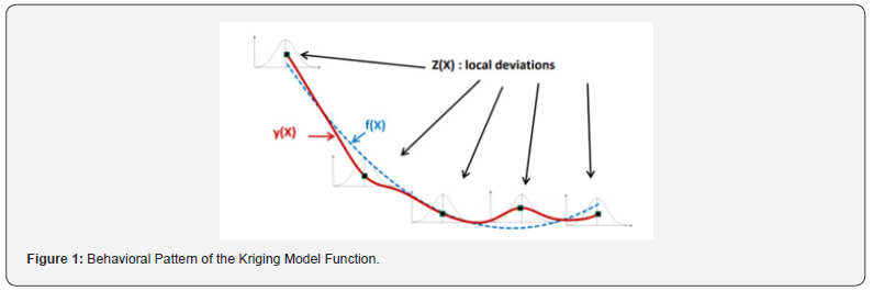
It is a multi-dimensional interpolation model that associates a polynomial model analogous to one of the standard response levels, which is stated as a comprehensive model of the design space, plus a detailed local deviation that can intercept design points of the model.

The method denotes the output parameter as a function of input variables as given below:

output = f (inputs) + z(inputs)

Where f is a quadratic polynomial function and z is the deviation term

Meanwhile, this model fits the contact surfaces at all design points, so it will always give appropriate goodness of fit criterion. Which has improved results than the standard response surface model, if the output elements are stronger and nonlinear. The major disadvantage is that fluctuations can occur on the response surface. Figure 1 shows the behavioral pattern of the function related to this model. where the behavior of the estimated function comprises a general function (f) combined with a local function (z).

Non-Parametric Regression Model

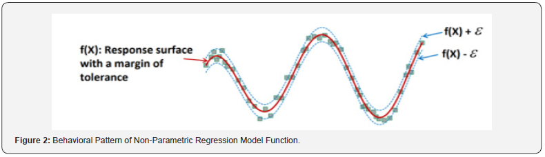
It tends to be a general class of RSM model, where the epsilon (Ԑ) tolerance forms a fine covering around the output response surface and spreads around it. This covering space should comprise all the design sample points. Instability regression is created to estimate the regression function directly, which means instability regression can directly study the effect of independent variables on a dependent parameter without notifying a particular function to create the relationship between the independent and dependent variables. Figure 2 shows the behavioral outline of the function related to the non-parametric regression model. The behavior of the predictable function consists of a principal response surfaces with a margin of tolerance on both side.

Neural Network Model

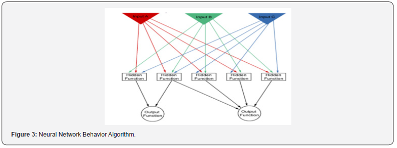
It represents a mathematical practice based on natural neural networks in the human brain, which connects every input variable to weights by arrows. Which can find the inactive or active hidden functions, that are the threshold elements allows the output function to connect or disconnect based on a set of their input variables. Finally, every time the procedure is repeated. It adjusts these weight functions to diminish the error between the response levels with the design points. Figure 3 shows the behavioral algorithm of the cellular network model, which consists of input variables, hidden functions, and output functions.

Sparse Grid Model

It is a type of adaptive response surface, which can continuously correct itself automatically. It usually needs extra design points than other methods. The capability of it is that it adjusts the design points only in the directions that requires. For which, it requires less design points to complete the same quality response level. This model is also fit for cases that contain multiple discontinuities.

Methods of RSM [14]

RSM is often a step-wise procedure where the response surface points remote from the optimum. This method focuses on the travel from the existing point to the optimum point with a sequence.

There are two methods for getting the optimum point:

i. The method of steepest ascent

ii. The method of steepest descent

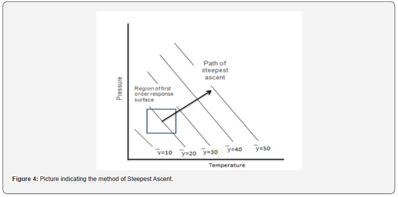
i. Method of Steepest Ascent: It is a course of moving consecutively in the direction of the extreme increase in the response to the optimum response, which is indicated in Figure 4.

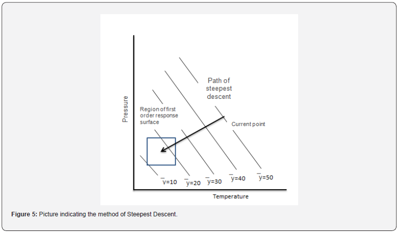
ii. Method of steepest descent: It is a course of moving consecutively to minimize the response, which is indicated in (Figure 5).

Types of response surface modeling [15-16]

i. Central Composite Design (CCD)

ii. Box-Behnken Design (BBD)

i. Central Composite Design (CCD)

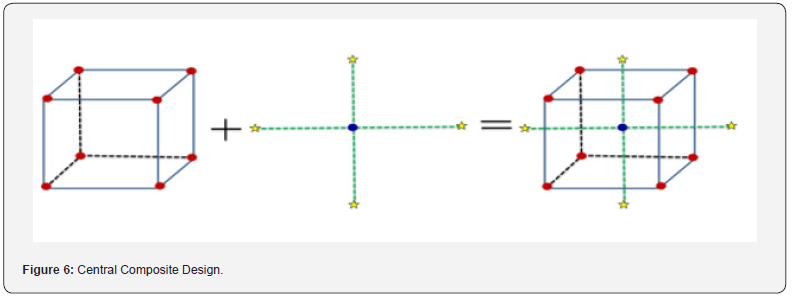
The central composite design is the most widespread and adaptable response surface design and maximum researchers pick this design. The central composite design was published by Box and Wison in the year 1951. A central composite design always has 2 levels and k influencing factors. It comprises axial points and center points. Initially, produce a 2^k factorial or a 2^k-p fractional factorial design, and then affix extra runs denoted to as axial points (Figure 6). The 2^k and 2^k-p part of the design permits to fit of first-order terms and relations. Similarly, the axial points help to the extra level required to fit the second-order model.

ii. Box-Behnken Design (BBD)

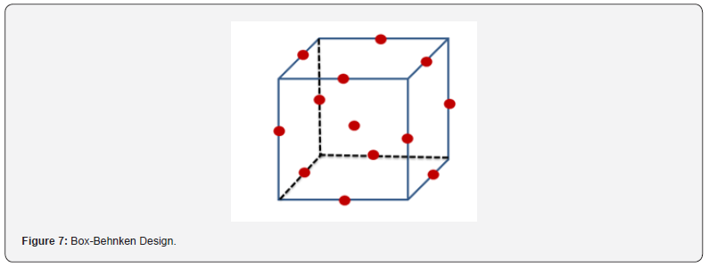
It is the famous response surface method for a three-level factor, suitable for the second-order model to the response. In 1960, Box and Behnken were first established this method. It is a blend of two-level factorial designs with incomplete block designs. The advantage of this design is it does not contain corner points, which means any points at the out of the cubic region formed by the two-level factorial level combinations (Figure 7).

Data analysis

After finishing the experimental work by a suitable RSM design, the output responses may be modelled and the data is fitted with polynomial equation to find the relation between the responses and factors studied. ANOVA is used to test the statistical significance of the model. ANOVA allows the decision of inclusion or exclusion of coefficient of linear terms, interaction terms and quadratic terms in the model based on p-value. If the p-value is less than 0.05 means the response is affected by the varying levels of the input parameters, and that terms have to include in the regression model or else if p-value is greater than 0.05 declares no effects of varying levels of input factors on response, and that should be eliminated from the regression model [17].

Multiple regression model can be adjusted by coefficient of determination values like R², adjusted R² and predicted R². The variation of output response based on the input factors will be explained by R² value. Addition of new terms to the regression model will increases the R² value. Adjusted R² is the modified version of R², which helps in the adjustment of terms in the regression model, adjusted R² get increased, if the added terms improve the model. Predicted R² indicates how well a regression model predicts output responses for new observations and is calculated by removing each observation from the data set systematically. R² is always higher than adjusted and predicted R² values. The difference between the predicted and adjusted R² values should be less than 0.2 in order to obey the fit statistics. Adequate precision measures signal to noise ratio and a ratio of greater than 4 is desirable which tells that the model can be used to navigate the design space. When the error provided by the regression model lack of fit is significantly lower than a random pure error (p-value > 0.05), it indicates that the regression model is well fitted. Lake of fit data must be non-significant and it can be estimated only when replicas usually for centra point are included in the experimental design [18].

Diagnostic plots [19]

a. Normal probability plot: These plots indicate whether the residuals follow normal distribution represented by a straight line. S-shaped curve indicates that transformation of response is necessary to provide better analysis.

b. Residual Vs. Predicted plot: A graph is plotted between residuals and predicted response values in ascending order denoted by a random scatter.

c. Residuals Vs. Run: This is a plot of residuals versus experimental run order denoted by a random scatter.

d. Predicted Vs. Actual: The plot is drawn between predicted versus actual response values.

e. Box-Cox plot for power transforms: This plot is for power transformation based on the best λ value and if a 95% confidence interval around this λ includes 1 then transformation is not recommended.

f. Residual Vs. Factor: This is a plot of residuals versus any factor of choice denoted by a random scatter. If the curvature effect is seen it indicates that the contribution of the independent factor is not taken into consideration.

g. Model graph [20]: To interpret the selected model various graphs are provided in the design expert software. For factorial designs, the most commonly used graphs are one factor, interaction, and cube. For response surface and mixture designs 2D Contour and 3D Surface plots are used.

h. Perturbation plot: These plots compare all factor effects at a particular point in design space and the response is plotted by varying only 1 factor over its range and keeping all other factors constant. The steepest slope or curvature indicates the response is sensitive to that factor and the flat line indicates the response is not affected by that factor.

i. One factor effects plot: These plots show linear effects by changing the levels (-1 : low, +1 high) of a factor and predicting the responses.

j. Interaction graph: These plots appear as two nonparallel lines which indicates that one factor effect depends on another factor level.

k. Contour plot: It is a 2D representation of response plotted against numeric factor combination which shows the relationship between responses.

l. 3D Surface plot: It is a contour plot projection which gives shape along with contour and color.

m. Cube plot: It shows the predicted values from the coded model for the combinations of -1 and +1 levels of any 3 factors.

Optimization by desirability functions approach

This approach finds a factor setting that provides the most desirable response. Each response is assigned a number between 0-1 for a completely undesirable to desirable or ideal response value. Finally overall desirability is obtained by combining the individual response desirabilities using a geometric mean [21].

Conclusion

RSM can be used for the approximation of both experimental and numerical responses. Two steps are necessary, the definition of an approximation function and the design of the plan of experiments. The success of RMS depends on an estimation of y at different locations in the response surface. Therefore, the experimenter can draw a conclusion about whether the system contains optimum or improvement in response. Before any experimenter starts the analysis of the response surface, the application of RMS first begins with investigation of factors or variables. In order to obtain an efficient experiment, unimportant independent variables need to be separated from important ones. One should never start an analysis of the surface until significant factors are identified. After that, the response surface study can start. Four steps for response surface analysis are (1) perform a statistically designed experiment, (2) estimate the coefficients in the response surface equation, (3) check on the adequacy of the equation (via a lack-of-fit test), and (4) study the response surface in the region of interest. Besides statistical and mathematical techniques the graphical representation of the response surface is also helpful in finding answers to problems. Due to broader applications in real-word problems, RMS will continue to attract statisticians, engineers, and scientists in order to develop, improve, and optimize new or existing products and processes.

To Know more about Global Journal of Addiction & Rehabilitation Medicine

Click here: https://juniperpublishers.com/gjarm/index.php

To Know more about our Juniper Publishers

Click here: https://juniperpublishers.com/index.php

Development And Preclinical Evaluation of Anti-Analgesic, Anti-Pyretic, Anti- Inflammatory and Antioxidant Potential of Polyherbal Formulation on Experimental Animal Model - Juniper Publishers

Cell Science & Molecular Biology - Juniper Publishers

Abstract

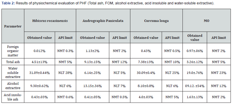
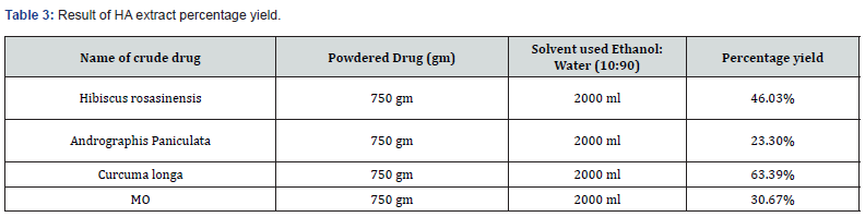
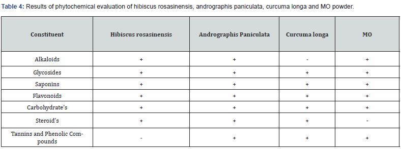
The concept of polyherbal formulation (PHF) was initiated via Ayurvedic and other traditional medicinal systems. Additionally multiple plants were used to develop the formulation and evaluated pharmacologically for their synergistic action as well as used to treat many diseases. In the present work we focused on the development and nonpharmacological as well as pharmacological evaluation of PHF on experimental animal model. The plant materials Hibiscus rosasinensis, andrographis paniculata, curcuma longa and moringa oleifera (MO) were collected. Furthermore processed for the evaluation of water soluble extractives, percentage yield, Phytochemical screening, angle of repose, loose and tapped bulk density, carr’s index, hausner’s ratio physiochemical parameters i.e. foreign organic matter, total as value, alcohol soluble extractive value, compressibility index, Hauser ratio, acute toxicity study, anti-analgesic activity such as thermal pain model, mechanical pain model, antipyretic activity, carrageenan induced inflammation as well as antioxidant activity respectively. Phytochemical screening Plant materials were identified and approved by the department of pharmacognosy Columbia Institute of Pharmacy, Raipur, Chhattisgarh, India. The outcomes were found that water soluble extractive of Hibiscus rosasinensis, andrographis paniculata, curcuma longa and moringa oleifera (MO) were 31.09±0.44%, 6.14±.25%, 30.09±0.4% and 19.0±.76%. The percentage yield was 46.03%, 23.30%, 63.39% as well as 30.67% respectively. Moreover, Phytochemical screening of plant materials revealed the presence of Alkaloids, glycosides, saponins, flavonoids, carbohydrate’s, steroid’s, tannins, and phenolic compounds. Data of angle of repose, loose and tapped bulk density, carr’s index, hausner’s ratio were seen 27.03, 0.34, 0.61, 11.97 and 1.11. Additionally acute toxicity was performed as per OECD guideline 423, no weight changes as well as no mortality after 24 h and no behavioral changes observed even at the maximum dose of 4000 mg/kg. Anti-analgesic activity was evaluated as per thermal pain model and mechanical pain model experimental animals were categorized into five groups, Group I treated with normal saline, Group II aspirin 150mg/kg (thermal pain model) & diclofenac sodium 150 mg/kg (mechanical pain model), Group III, IV as well as V were received PHF graded dose reaction time increases with increasing in dose. Antipyretic activity was evaluated on brewer’s yeast induced animal model rectum temperature was reduced with increasing the PHF dose, comparative study was done Paracetamol used as standard. Furthermore, carrageenan induced inflammation was revealed that paw edema size reduced with increasing the dose of formulation. Antioxidant evaluation was done using 2,2-diphenyl-1-picrylhydrazyl radical (DPPH.) assay and oligomeric proantho cyanidins (OPC) was used as a standard, PHF shows antioxidant activity on dose dependent manner furthermore results were shown in the graph a) and b) respectively. The present information on the PHF development and evaluation of the Hibiscus rosasinensis, andrographis paniculata, curcuma longa and moringa oleifera (MO) revealed the qualitative, quantitative, and pharmacological parameters provide the huge information to the identity and to determine the quality and purity of the plant material in the future.

Keywords: Hibiscus Rosasinensis; Andrographis Paniculata; Curcuma Longa and Moringa Oleifera (MO); Polyherbal Formulation; Anti-Analgesic; Anti-Pyretic; Anti-Inflammatory And Antioxidant

Abbreviations: PHF: Polyherbal Formulation; MO: Moringa Oleifera; OPC: Oligomeric Proantho Cyanidins; FOM; Foreign Organic Matter

Introduction

All living things experience pain and inflammation which can be brought on by physical, chemical, or biological factors. Inflammation is often characterized by erythema, swelling, heat, discomfort, and dysfunction. Analgesics are painkillers but they can have several adverse effects such as respiratory depression, apnea, nausea, vomiting, physical and mental illness etc. [1,2]. When used long-term or in high dosage, cell injury and the synthesis of inflammatory mediators such as platelet-activating factors (LTB4) and arachidonic acid prostaglandins (PGE2) in migratory cells are the outcomes of local tissue damage. Neu- trophils and macrophages, which migrate and infiltrate organs, release pro-inflammatory cytokines such as IL-1𝛽 and TNF-𝛼. Folk medicine comprises medical aspects of traditional knowledge that developed over generations within the traditional system beliefs of various societies, including indigenous peoples before the era of modern medicine. While Polyherbal formulation (PHF) is the use of multiple herbs in a therapeutic preparation. The concept was found in ayurvedic and other traditional medicinal systems where multiple herbs in a meticulous ratio may be used in the treatment of diseases [3]. Nowadays most diseases possess due to excessive prostaglandins and oxidants produced in the body which modifies physiology of body. The management of prostaglandins and antioxidants through the herbal’s formulation is a rational approach to preventive health care. The importance of disease prevention is recognized by ayurveda through experience accumulated over centuries. Hibiscus rosasinensis, andrographis paniculata, Curcuma longa and moringa oleifera (MO) in the ratio of 1:1:1:1. Antioxidant and immune-stimulating effects of M.O. have already been established in animal models [4].

Materials and Methods

Drugs and Chemicals used

Methanol 95%, normal saline (Merck Ltd India), acetic acid (New arihant chemicals mumbai ,india,), brewer’s yeast and carrageenan (Bayers Pvt Ltd). Tramadol, aspirin, diclofenac sodium, paracetamol (Cipla Pharmaceutical Industry India) and other chemicals were used as well as procured of analytical grade.

Collection, Identification and Authentification

The fresh flowers, leaves, roots, and fruits of Hibiscus rosasinensis, andrographis paniculata, curcuma longa and moringa oleifera (MO) were collected in june, 2021 from Raipur, Chhattisgarh, India. The plants were identified and authenticated by Dr. S. Prakash Rao, Department of Pharmacognosy, Columbia Institute of Pharmacy, Raipur, Chhattisgarh, India, 492001.

Physiochemical Evaluation

All plant parts were dried, crushed and converted into fine powders with the help of mixer and grinder there after quality assessment of plant materials were done as per the standard protocols of Ayurvedic Pharmacopeia of India (API). Different parameters were tested with the methods described in API [5].

Foreign Organic Matter (FOM)

As per API, FOM is described as any material that consists of part of organ or organ part from which the drug is derived. The plant should be free from any unfamiliar particle like dust, insects, faecal matter etc. The percentage of foreign matter should not be more than the limit prescribed in monograph. There should not be any contamination in drug material used for PHF [6].

Procedure

750 gm of plant materials were weighed and spread as a thin layer and was inspected first with naked eyes thereafter by using lens (6x). The entire FOM were Separated, weighed and percentage was deliberated.

Determination Of Total Ash Value

3.0 gm of dried powered mixed sample was weighed in silica dish, and it was incinerated at a temperature not exceeding 450°C until it gets free from carbon. The incinerated material was cooled, weighed and percentage of ash was calculated with reference to air dried drug. The determination of Acid insoluble ash value Ash obtained was boiled with 25 ml of dil. HCL for 5 minutes filtered and insoluble matter was collected in crucible and washed with hot water and ignited till constant weight. The percentage of acid insoluble ash was calculated with respect to air dried drug [7].

Determination of Alcohol Soluble Extractive Value

5gm of powdered drug was macerated with 100 ml of alcohol in cork fitted conical flask. Solution was shaken frequently for 6 hrs and was allowed to stand for 18 hrs. After 18 hr. content was filtered and 25 ml of filtrate was evaporated to dryness in a shallow dish at 105°C to constant weight and percentage of alcohol soluble extractives was calculated with reference to air dried drug.

Determination of Water-Soluble Extractives

5gm of powdered drug was macerated with 100 ml of water in cork fitted conical flask. Solution was shaken frequently for 6 hrs and allowed to stand for 18 hrs. After 18 hr. content was filtered and 25 ml of filtrate was evaporated to dryness in a shallow dish at 105°C to constant weight and percentage of water-soluble extractives was calculated with reference to air dried drug. The data generated in respect of the above findings will be used as in-house standards.

Preparation of Hydro-Alcoholic (HA) Extracts and Percentage Yield Estimation

Dried powder was processed in order to prepare the PHF, about 750gm of Hibiscus rosasinensis (flower, leaves), 750gm of andrographis paniculata (flower, leaves, roots), 750gm of curcuma longa (flower, roots) and MO (flower, leaves, fruits) powders were soaked overnight separately in 1500ml of Petroleum Ether (PE). After 3 days the suspension was filtered, and PE was to be evaporated overnight. Again, the dried powders were separately resuspended in a Stoppered container with the HA solvent. Allowed to stand at room temperature (RT) for a period of 7days. Additionally, extract was concentrated to dryness in a rotary evaporator (Buchi type) under reduced pressure and controlled temperature (37-40℃) to get percentage yield [8].

Phytochemical Screening

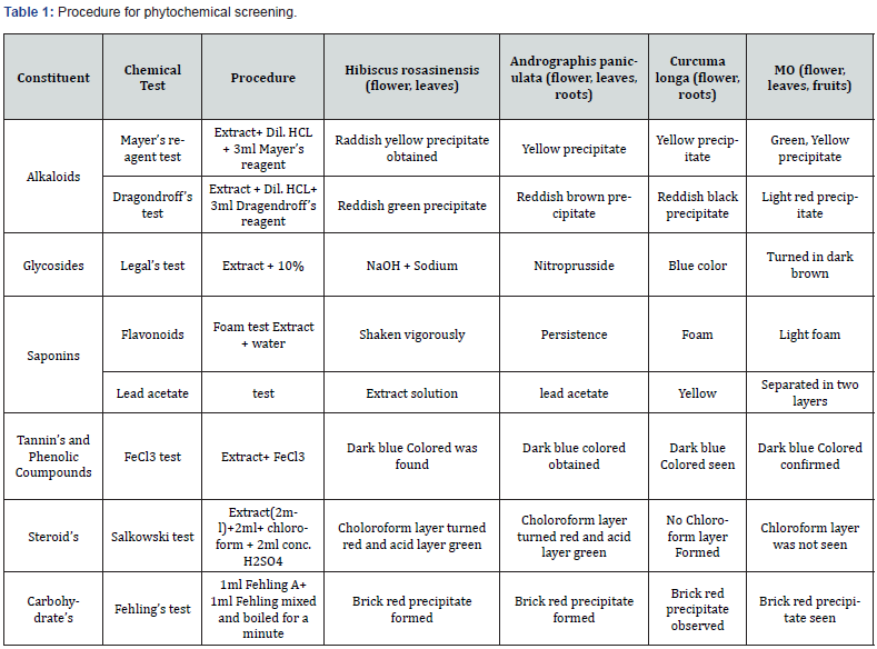
Crude extract of plants was subjected to different chemical tests to detect the presence of various phytochemical constituents as per procedure adopted in literature. The details are incorporated below in table 1, the entire chemical test was discussed in results table 2,3 [9].

Design and Development Of PHF

Extracts of four plants Hibiscus rosasinensis, andrographis paniculata, curcuma longa and moringa oleifera (MO) formulation have been made by blending the extracts in ration 1:1:1:1. Evaluation of Polyherbal formulations Prepared PHF was evaluated on following parameters [10].

Angle Of Repose

The angle of repose was determined by using the funnel method. The accurately weighed blend was taken in a funnel. The height of the funnel was adjusted in such a way that the tip of the funnel just touches the apex of the heap or head of blend. The drug excipient blend was allowed to flow through the funnel freely onto the surface. The diameter of the powder cone was measured, and angle of repose was calculated using the following equation:

tan θ = h/r

Where, h = height of powder cone formed, r = radius of the powder cone formed

Loose Bulk Density

Apparent bulk density was determined by pouring a weighed quantity of blend into graduated cylinder and measuring the volume and weight.

LBD = Weight of the powder / volume of the packing.

Tapped Bulk Density

It was determined by placing a graduated cylinder, containing a known mass of drug excipient blend. The cylinder was allowed to fall under its own weight on to a hard surface from the height of 10cm at two second intervals. The tapping continued until no further change in volume was noted.

TBD = Weight of the powder/vol of the tapped packing

Compressibility Index

The Compressibility index of the powder was determined by Carr’s compressibility index.

Compressibility index (%) = (TBD-LBD) x 100/TBD

Hausner Ratio

It is the measurement of frictional resistance of drug and ideal range should be 1.2-1.5. It is determined by using the following formula:

Hausner ratio= TBD / LBD

Acute Toxicity Study of PHF As Per OECD Guidelines

Preparation of Formulations

For dosing 100 ml of each formulation was prepared by dissolving 5gm of formulation in 100 ml of distilled water (So, 1ml contain 50 mg of drug).

Experimental Animals

Healthy male albino wister rat were taken weight ranging from 175-250gm. The animals were procured and kept at the animal house of the Columbia Institute of Pharmacy, Raipur, Chhattisgarh, India. Animals were reserved in a neat and clean atmosphere in polypropylene cages, under 12 h light and dark cycles. The room temperature (RT) was maintained at 24 ± 0.40C with controlled humidity. Animals were fed in strict hygienic conditions with a rodent pellet diet and water ad libitum. The experiments on animals were performed and approved as per the guidelines of the Animal Ethics Committee. All the animal experiments were carried out according to the Committee for the Purpose of Control and Supervision of Experiments on Animals (CPCSEA) guidelines, Regd. No. 0310/PO/ReBi/S/20/01/CPCSEA.

Acute Toxicity Study of PHF

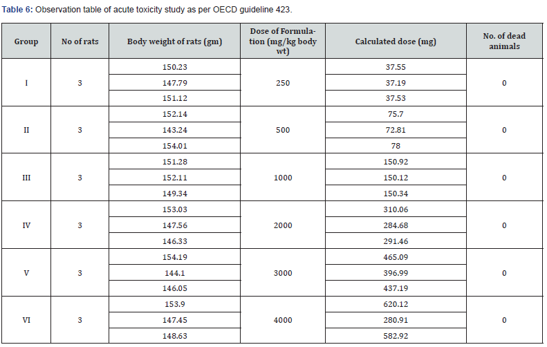
Acute toxicity studies were carried out in adult female albino rats weighing between 130-180 gm by Acute Oral Toxicity method of OECD Guideline 423. They were administered (orally) with varying doses (250, 500, 1000, 2000, 3000 and 4000 mg/kg body weight) for each of six formulations. Animals were divided into 6 groups of three animals each and were acclimatized for 5 days. Prior to dosing animals were kept fasted overnight and next day each formulation was administered orally at a dose level of 250, 500, 1000 and 2000 mg/kg body weight. Rats were observed for clinical signs of toxicity continuously for 2 hours and occasionally for further 4hours for general behavioral and finally for any mortality after 24 hours till 14 days. No mortality was observed during a time period of 14 days [11].

Analgesic Activity

Thermal Pain Model (Tail Flick)

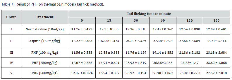
Rats were categorized in Group I (Control: Normal saline), Group II treated with Aspirin, 150 mg/kg; Group III, IV & V were given PHF treatment 250 and 500 mg/kg orally one hour before beginning of the experiment. The tip of the tail was immersed in tail flick algesimeter (50.0 ± 1.0 °C) and observed for response. Data were noted at 0, 15, 30, 60, 120, and 180 min in tabular format.

Mechanical Pain Model (Eddie’s Hot Plate)

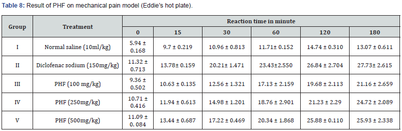
Animals were grouped consequently Group I (Control: Normal saline), Group II Diclofenac sodium (150 mg/kg); Group III, IV & V treated with PHF 250 and 500 mg/kg. We placed the rats’ right paws on the eddies hot plate and spontaneous withdrawal reflex was recorded at 0, 15, 30, 60, 120, and 180 min respectively.

Antipyretic Activity

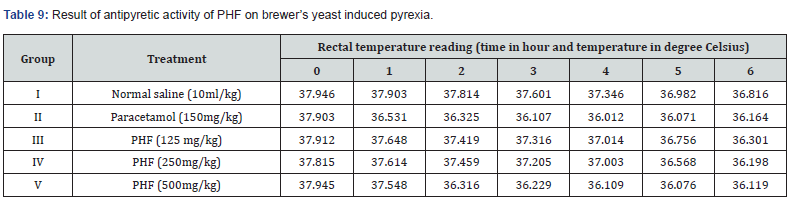
In this present work we used Brewer’s pyrexia for the elevation of body temperature in animals. They received 20% w/v of brewer’s yeast suspension 10 ml/kg. Furthermore, animals were randomized into five groups, Group I was considered as controlled group, Group II was treated with 150mg/kg paracetamol, Group III, IV & V were given 125, 250 and 500 mg/kg of PHF. The temperature of rectum was noted at the time interval of 0, 1, 2, 3, 4, 5 and 6 h respectively.

Carrageenan Induced Inflammation (Paw Edema)

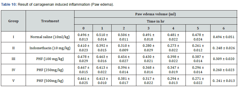
Animals were grouped accordingly Group I Control (Inflammation control), Group II was treated with Indomethacin 10 mg/kg and Group III, IV & V were given orally 100, 250 and 500 mg/kg of PHF 30 minute earlier than carrageenan injection. Moreover, each animal’s left paw was injected 2.0% w/v carrageenan after 0, 30, 1, 2, 3 and 4h every rat’s paw volume was measured carefully using water paleothermometer. Size of edema were noted down by means of A and B where A is before the inducing agent treatment as well as B is after induction [12].

Antioxidant Activity

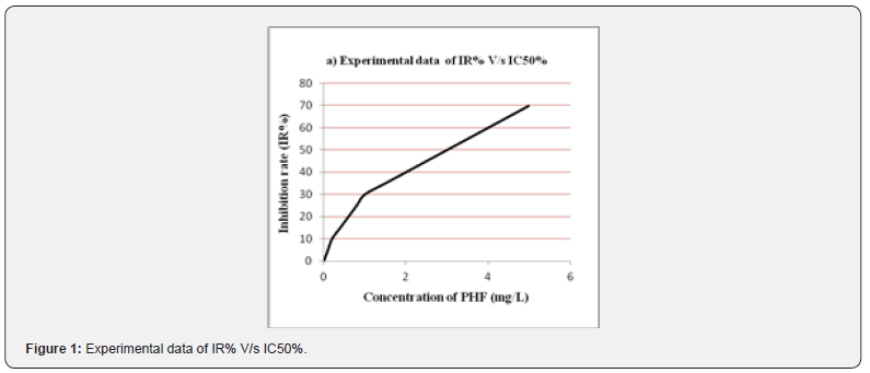
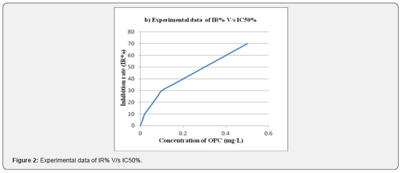
The free radicals scavenging property of PHF was determined by 2,2-diphenyl-1-picrylhydrazyl radical (DPPH.) assay and oligomeric proantho cyanidins (OPC) was used as a standard for the comparative study of PHF extract. Furthermore, a 50% inhibition rate in the corresponding concentration is known as IC50. Hence the significance of IC50 was calculated by comparing the values of sample concentration and inhibition rate of PHF [13].

Result and Discussion

Physiochemical Evaluation Of PHF

The data of all determinations were summarized in Table 1, parameters incorporated such as foreign organic matter, total ash, acid insoluble ash, alcohol as well as water soluble extractive of PHF; preparation was found under ayurvedic pharmacopoeia confines. (Table 2)

Percentage Yield of HA Extract

HA extract of powdered crude drug were obtained after soaking for the three days. Furthermore, processed through the butchi rotavapour, percentage yield statistics information was given in Table 3.

Phytochemical Evaluation Of PHF

Extract of crude drugs was processed for some special identification tests to distinguish the presence of different chemical components. Additionally, evaluation parameters i.e., Alkaloids, glycosides, saponins, tannins, phenolic Coumpounds, steroid’s as well as Carbohydrate’s result were described in Table 4.

Design, Development, and Evaluation Parameters Of PHF

PHF was prepared as per standard technique as per previously reported in literature, which targeted each site in the body. Furthermore, formulation is helpful in minimizing analgesic, pyretic, inflammation as well as having strong ability to scavenge free radicals. Additionally evaluated on the parameters i.e., Angle of repose, loose bulk density, tapped bulk density, carr’s index as well as hausner’s ratio respectively figures were given in Table 5.

Acute Toxicity Study of PHF

Phytochemical screening of PHF established that it be full of Alkaloids, glycosides, saponins, flavonoids, carbohydrates, steroid’s, tannin’s along with phenolic compounds as per API. Furthermore, acute toxicity study of PHF was estimated as per OECD guideline 423, formulation lead to no weight changes as well as no mortality after 24 h and no behavioral changes observed even at the maximum dose of 4000 mg/kg statistical analysis given in observation Table 6.

Evaluation of Anti-Analgesic Activity

Thermal Pain Model (Tail Flick)

Throughout the observation period normal saline, aspirin 150 mg/kg and PHF graded dose 100, 250 and 500mg/kg were administered. Values were compared as well as revealed that tail flicking time is directly proportional to dose, given in Table 7.

Mechanical Pain Model (Eddie’s Hot Plate)

During the 180h of observation period experimental animals were administered normal saline 10ml/kg, diclofenac sodium 150mg/kg and PHF 100mg/kg, 250mg/kg as well as 500mg/g body weight. Consequences observed that reaction time increases in dose dependent manner, given in Table 8.

Evaluation of Antipyretic Activity

Pyrexia was induced by brewer’s yeast, reduction of rectal temperature by different doses of paracetamol and PHF were noted on Table 9. Furthermore, evidence was seen that PHF reduces body temperature in a dose dependent manner.

Carrageenan Induced Inflammation (Paw Edema)

The experimental animals were induced using carrageenan as well as treated with normal saline 10ml/kg, indomethacin 10 mg/kg and PHF 100, 250 and 500 mg/kg body weight respectively. Hence, results were elevated that size of induced paw edema gradually decreases in the dose dependent manner; values were given in Table 10.

Evaluation Of Free Radicals Scavenging Property

The PHF of Hibiscus rosasinensis, andrographis paniculata, curcuma longa and MO confirmed that the scavenging of DPPH free radicals and a maximum scavenging activity was depends on the concentration. Still data were recorded at a concentration of 1, 2, 3, 4, 5 and 6 mg/L PHF, respectively. OPC, with the strong ability to scavenge free radical, was used as the standard to estimate the antioxidant activity of PHF. As per (Figure 1,2) the assessment of IR greater than before along with the concentration added. Furthermore, the IC50 value of PHF and OPC were established that 3.0mg/L as well as 0.3mg/L respectively. Therefore, the antioxidant activity of extracts from 1 mg PHF was approximately equal to 0.1 mg OPC.

To Know more about International Journal of Cell Science & Molecular BiologyClick here: https://juniperpublishers.com/ijcsmb/index.php
To Know more about our Juniper PublishersClick here: https://juniperpublishers.com/index.php

Efficiency Modeling using the Mirror Surface of Heliostats in a Solar Power Tower - Juniper Publishers

 Material Science - Juniper Publishers

Abstract

Analyzing the geographical location and climatic conditions of Turkmenistan, we conclude that solar energy is a priority among all renewable sources since the duration of sunny days in the country is from 270 to 320 days a year. Development, creation of large-scale solar power plants and use in remote desert regions of Turkmenistan is an urgent problem. The article considers the possibilities of creating a solar power plant based on a tower-type layout. The modes of the optical system in the natural and climatic conditions of Turkmenistan are calculated using a mathematical model, the coefficient of efficiency of using the mirror surface of the installation and the distribution of the level of instantaneous local values are determined. Figure 1 shows the movement of the Sun in the sky, which varies depending on the time of year. The results of the study show that the maximum increase in the energy efficiency coefficient can be achieved with the location of solar panels perpendicular to solar radiation with the dense placement of heliostats on the north side of the tower, then energy efficiency will increase by 25-40% in summer and 10-15% in winter.

Keywords: Solar energy; Tower solar power plant; Efficiency coefficient; Mirror surface; Heliostat; Optical system; Turkmenistan

Introduction

In the 21^st century, humanity faced an acute problem of fuel for the power supply of various industrial and agricultural facilities. The reserves of minerals on Earth are not unlimited, the use of nuclear energy entails the danger of accidents, man-made disasters, and problems with the disposal of production waste. Against this background, the widespread use of renewable energy resources (RES) is of great interest. Turkmenistan, due to its geographical location and climatic features, is interested in the development of these energy sources.

The Law of Turkmenistan “On Renewable Energy Sources” regulates the relations between the state, producers and consumers, as well as the process of supplying equipment, installations and technologies for the use of renewable energy sources [1,2]. The Law outlines the main goals of using RES, in particular, reducing the growth of anthropogenic pressures on the environment and countering climate change, improving the quality of life and maintaining public health by reducing the growth of planetary pollution. The introduction of renewable energy resources into the fuel and energy complex will reduce the cost of transporting electricity, reduce the anthropogenic load on the environment and improve the social and living conditions of residents in remote areas, in this case, residents of the Karakum desert zone. All this undoubtedly indicates the extreme relevance of this topic [1-3]. The potential of solar energy is a ball of hydrogen and helium, in which continuous thermonuclear reactions occur, as a result of which energy is released with a temperature of t≈ 6000 o and radiant energy of 18000 billion kW, while the energy intensity on the Earth’s surface is 70-80 thousand kW / m². But the intensity of solar radiation on the Earth’s surface depends on the natural and climatic features of the area, geographic latitude, air transparency, time of day and year, as well as altitude above sea level [3]. The gross potential of solar energy in the territory of Turkmenistan is estimated per square meter in the range from 1687.7 to 1897.2 kWh/m² per year, the technical potential for heat production is from 1177.1 to 1296.78 kWh/m² per year.

The amount of solar energy supplied to a horizontal surface varies depending on the natural and climatic conditions of the country’s region. The duration of sunshine at any point depends on the length of the day, cloudiness and increases from approaching the equator. However, the latitudinal distribution of sunshine is often disturbed due to the presence of clouds due to the peculiarities of atmospheric circulation, and fogs in coastal zones. The duration of sunshine on the territory of Turkmenistan varies depending on the season of the year in hours: in winter from 107 to 120, in spring 146-282, in summer 331-352, and in autumn 160-293. The total duration of sunshine is 2680 hours, the average daylight time is 8 hours 40 minutes per year. The average sunrise time is 6 hours 50 minutes, the average sunset time is 17 hours 25 minutes.

The potential of solar energy is the sum of the duration of solar radiation during the year and the total solar radiation incident on a horizontal surface. It is possible to increase the amount of solar radiation by changing the angle of inclination of the receiving surface. The maximum magnification will be achieved if the solar tracking panels are placed perpendicular to the solar radiation [3]. In the efficient operation of a solar power plant, the most important role is played by the optimal orientation of the solar radiation receiver with three main angles: the latitude of the receiver location φ , the hour angle ω and the declination of the Sun δ, shown in figure 1 for clarity.

Figure 1 shows the latitude, φ is the angle between the line connecting point A with the center of the Earth 0, and its projection onto the equatorial plane. The hour angle, ω, is the angle measured in the equatorial plane between the projection of the line OA and the projection of the line connecting the centers of the Earth and the Sun. Angle ω = 0 at solar noon; per hour corresponds to 15°. The declination of the sun, δ, is the angle between the line connecting the centers of the Earth and the Sun and its projection onto the equatorial plane. The declination of the sun continuously changes throughout the year: from -23°27’ on the day of the winter solstice on December 22 to +23°27’ on the day of the summer solstice on June 22 and is equal to zero on the days of the spring and autumn equinoxes (March 21 and September 23) [3-6].

Based on this, the position of the Sun relative to the Earth continuously changes during the year and day, then in order to obtain the maximum possible power density of solar radiation, the angles must also change accordingly, therefore, continuous tracking of the movement of the Sun is necessary. However, as numerous studies have shown, the use of automated tracking systems increases the cost of solar installation. In this regard, stationary solar receivers are the most effective for low-power solar installations. The method with a fixed orientation of the panels for the entire period of operation has the lowest energy efficiency, but it is easy to implement.

Using innovative methods, it is possible to calculate the level of specific insolation for each day of the month of the year under average meteorological conditions. The goals and objectives of the study are to carry out an overview analysis of modern structures, develop a model of a solar tower station, and optimize the operating modes of the optical system of a solar power station using computer simulation. The scientific novelty lies in the calculation of the efficiency factor for the use of a mirror surface in the heliostat field of a solar tower power plant in Turkmenistan. The calculation method is based on theoretical calculations using geometric and optical elements to create a model of a tower solar station.

The day in the middle of the month was considered a typical day. Multiplying the specific daily energy of solar radiation by the number of days in a month, we obtain the specific monthly energy of solar radiation.

Solar Electric Station of Tower Type (TSPS)

The design of the solar power tower type consists of a tower of various heights depending on the power (from 18 to 24 m), and a black water tank, which is located at the top of the tower. Black color serves for better heat absorption. Outside there is a turbogenerator, from which pumps supply water to the tank. Around the tower are mirrors – heliostats (Figure 2) [5,6].

The principle of operation of heliostats is related to the general mechanism for tracking the position of the sun in the sky. The main task of the tracking mechanism is to ensure that heliostat mirrors located in a certain area around the station reflect the sun’s rays exactly into the steam generator. The power of a tower solar power plant depends on the number of installed heliostats. As a result, the concentration of solar radiation increases from the number of heliostats and the water temperature in the steam generator reaches up to 700°C, while powerful steam is formed that rotates the electric generator, electricity is generated and the efficiency of such solar power plants reaches up to 20% [5,6]./p>

Research Methodology

Mathematical research methods can reduce the search time, help in making adequate decisions, and increase the reliability of the entire system and the efficiency of the station [7-10].

One of the main tasks of designing solar tower stations is the rational arrangement of the optical system of mirrors. For their smooth operation, it is necessary to take into account a number of requirements, factors and limitations [10]. For example, to achieve a high radiation flux concentration factor, it is necessary to place a large number of mirror reflectors in the smallest possible area. However, the dense arrangement of specular reflectors in the specular field leads to their mutual shading [7-10]. Thus, the loss of solar radiation flux in the optical system really affects the efficient operation of solar power plants, as well as the operation of solar furnaces.

To implement the task, a mathematical model was compiled that allows a comparative analysis and selection of layout options for the optical system of a tower-type solar power plant [10]. For the rational use of optical systems, determining the efficiency, and the efficiency of using the mirror surface of heliostats in a tower solar power plant, a mathematical model has been compiled [7- 10]. When developing a computational scheme for a mathematical model of the operation of the fields of mirror reflectors of a solar power plant, we took into account the continuous coincidence of the normal vector N to the mirror and the bisector of the plane angle, which is located between the heliostat and the sun and the heliostat and the receiver.

The position of the mirror reflector of the heliostat is determined by the vectors Nj, the ratios of the vectors are shown in the geometric diagram (Figure 1). Applying the dot product rule for the i-th heliostat at a given time, is equal to the vector cosine of half the angle:

Here’s the expression for the cosine of a double angle:

cozy cosine coefficient is the efficiency optical system of solar SES.
From equation (1) and (3) we write:

Now, for the numerical implementation of the algorithm for calculating the values of the efficiency of the optical system of a solar station on a computer, we present the vector expression of the cosine coefficient of equation (4) in the form of a coordinate expression [7-10].

In the local Cartesian coordinate system XYZ, the components of the unit vector of the Sun have the form:

where X is the south side; Y is the east side; Z is the zenith; β-latitude of the location of the BSES, β=37 - 43 s.l. - for Turkmenistan; δ- the angle of inclination of the terrain is determined by the formula:

Ω- the hour angle is determined by the formula:

Where ω-the angular velocity of the Earth’s rotation is determined by the formula:

where τ- solar time, in hours, calculated from astronomical noon.

From figure 1, the components of a single vector in the XYZ coordinate system for individual heliostats are determined by the following formula:

In this formula, we make the following simplifications and assume that the first heliostat is located on the XZ plane, then the aiming coordinates focused at the tower point for all heliostats will be:

Where H is the height of the tower, H = 70 cm; r is the radius of the heliostat field, r = 110 cm.

Then in equation (9) we obtain the components Rxl in the following form

We determine the coefficient η for all mirror reflectors of a heliostat of a tower type, thus, we find the efficiency of using heliostats according to the formula:

Equation (11) shows that the efficiency factor for using the mirror surface η of heliostats depends on the angular variables and the distribution of its values over the field is uniquely determined by linear coordinates [7-10].

Research Results and Conclusion

In this research work, we analyzed the results of optimizing and modeling the operating modes of the optical systems of solar furnaces and a power plant based on solar energy using the developed and built mock-up of a tower-type power plant.

Mathematical modeling of the operating modes of the optical system of the specified power plant has been carried out. The coefficient of efficiency of using the mirror surface η was determined for all heliostats. Figure 1 and the mathematical model show that the quantitative and qualitative indicators of the distribution of instantaneous local values change depending on the position of the sun in the sky. The obtained results of the mathematical model confirm the efficiency of using the mirror field of heliostats for different times of the day. The distribution of instantaneous local values is constantly changing in different periods of the operation of the optical system..

a) As a result of calculations and observations, we conclude that the maximum increase in the energy efficiency coefficient can be achieved in summer by 25-40%, and in winter by 10-15%, these results are obtained under the condition that the heliostats are located perpendicular to the solar radiation and the heliostats are densely placed on the north side of the tower.

To Know more about Juniper Online Journal Material Science
Click here: https://juniperpublishers.com/jojms/index.php

To Know more about our Juniper Publishers
Click here: https://juniperpublishers.com/index.php

Application of Chicken Feather Fiber in Textile Industry: A Mini Review - Juniper Publishers

 Fashion Technology & Textile Engineering - Juniper Publishers

Abstract

Sustainability and environmental preservation are gaining significance in the textile industry. Feathers, an ever-present byproduct, are a promising environmental friendly textile alternative. This brief review covers poultry feather fiber in textiles. Chicken feather fibers (CFF) are composed of keratin and are biodegradable, strong, and lightweight. These characteristics make them desirable for textiles. Using mechanical, chemical, and enzymatic extraction and modification strategies, this article optimizes chicken feather fibers for textile use. Feather fibers can be incorporated into composites, filaments, nonwoven textiles, and coatings. They are hypoallergenic and biocompatible and have medical and healthcare applications. The carbon footprint and textile refuse of the industry are addressed. For widespread application, processing efficiency and scalability issues must be resolved. Feather fibers have potential. This brief analysis demonstrates that poultry feather fibers can be an environmentally friendly and sustainable textile industry option. This renewable resource has the potential to revolutionise the textile industry and promote sustainability and circularity.

Keywords: Textile; Chicken Feather Fiber; Livestock; Renewable; Sustainable Development

Introduction

The textile industry, one of the world’s largest and most visible, has historically relied heavily on materials that are resource-intensive and often environmentally hazardous [1]. The textile industry, like many others, has been feeling the pressure in recent years to adopt more environmentally friendly and sustainable practices. The growing number of eco-conscious individuals is largely responsible for this shift in perspective. As a result of this shift in thinking, scientists have begun exploring creative alternatives to traditional textile materials like the fiber obtained from chicken feathers. This paradigm change has specifically stimulated research into novel substitutes for traditional textiles [2,3].

Chicken feathers have gained a lot of attention recently due to their potential uses in the textile industry and their unique properties. Feathers from chickens are a common leftover from the poultry business. These feathers are biodegradable, strong, and incredibly light. Keratin, a protein also present in hair, nails, and horns, is the main component of these feathers. The textile industry is increasingly interested in acquiring materials that are sustainable and environmentally responsible, and because to their inherent features, they present an enticing option [4].

The goal of this article is to provide a comprehensive overview of the many applications of chicken feather fiber in the textile industry [5]. The processes of extracting and altering chicken feather fibers, as well as the various applications of these fibers in textile production, are only a few of the many issues explored. It also considers the environmental impacts and industrial challenges associated with using this cutting-edge material in textile manufacturing [6].

The textile business is constantly developing and changing to accommodate the needs of an increasingly eco-conscious clientele [7]. The industry is committed to both innovation and sustainability, and as part of this process, it is investigating unconventional materials like chicken feather fiber. In the quest for more sustainable textile production, chicken feather fiber has the potential to be a game-changer, and this article provides a thorough reference for understanding that potential [8].

Advantages of CFF in textile industry

CFF offers several advantages when used in Textile industry. Some of them are highlighted in figure 1.

Conclusion

Finally, the utilization of chicken feather fibers within the textile industry exhibits considerable potential and has great promise. This sustainable and ecologically conscious alternative to conventional textiles not only addresses the issue of poultry waste management, but also offers numerous additional advantages. The utilization of chicken feather fibers in fabric production offers notable advantages due to their lightweight and robust nature. These fibers possess the potential to be combined with various materials, resulting in fabrics that exhibit enhanced thermal insulation properties and improved moisture-wicking capabilities. Furthermore, they are a commendable option due to their accessibility and affordability. Despite the existing challenges related to processing and scaling, the continuous investigation and emergence of novel concepts within this domain indicate a promising outlook for the utilization of chicken feather fiber in revolutionising the textile industry, hence enhancing its sustainability, and reducing its environmental impact.

To Know more about Current Trends in Fashion Technology & Textile Engineering
Click here: https://juniperpublishers.com/ctftte/index.php

To Know more about our Juniper Publishers
Click here: https://juniperpublishers.com/index.php