Further Developments on the T-Transmuted X Family of Distributions II-Juniper Publishers

Biostatistics and Biometrics Open Access Journal

 

We review the exponentiated generalized (EG) T-X family of distributions and propose some further developments of this class of distributions [1].

AMS subject classification: 35Q92, 92D30, 92D25.

Keywords:T-XW family of distributions; Transmuted family of distributions; Exponentiated

Abbrevations: EG: exponentiated generalized; QRTM: Quadratic Rank Transmutation Map;

Introduction

Transmuted family of distributions

According to the quadratic rank transmutation map (QRTM) approach in Shaw W, et al. [2], the CDF of the transmuted family of distributions is given by

Where, 11λ−≤≤ and ()Gx is the CDF of the base distribution. When 0λ= we get the CDF of the base distribution

Remark 1.1. The PDF of the transmuted family of distributions is obtained by differentiating the CDF above.

A plethora of results discussing properties and applications of this class of distributions have appeared in the literature, and for examples see Faton Merovci, et al. [3] and Muhammad Shuaib Khan, et al [4].

T-XW family of distributions

This family of distributions is a generalization of the beta-generated family of distributions first proposed by Eugene et al. [5]. In particular, let ()rt be the PDF of the random variable T∈[a,b] ,−∞ ≤a< b ≤ ∞ and let WF((x)) be a monotonic and absolutely continuous function of the CDF F(x) of any random variable .X The CDF of a new family of distributions defined by Alzaatreh et al. [6] is given by

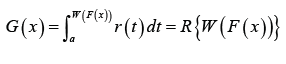
Where R(⋅) is the CDF of the random variable T and a≥ 0

Remark 1.2. The PDF of the T-X(W) family of distributions is obtained by differentiating the CDF above

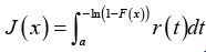
Remark 1.3. When we set W(F(x)):=-ln(1-F(x)) then we use the term “T-X Family of Distributions” to describe all sub-classes of the T-X(W) family of distributions induced by the weight function W(x):=-ln(1-x) A description of different weight functions that are appropriate given the support of the random variable T is discussed in Alzaatreh A, et al. [6]

A plethora of results studying properties and application of the T-X(W) family of distributions have appeared in the literature, and the research papers, assuming open access, can be easily obtained on the web via common search engines, like Google, etc.

T-Transmuted X family of distributions

This class of distributions appeared in Jayakumar K, et al. [7]. In particular the CDF admits the following integral representation for a≥0

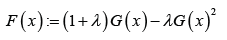
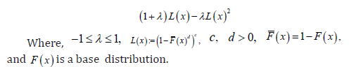
Where ()rt is the PDF of the random variable T and ()Fx is the transmuted CDF of the random variable ,Xthat is,

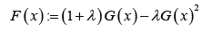
Where -1≤λ≤1 and ()Gx is the CDF of the base distribution.

Remark 1.4. The PDF of the T-Transmuted X family of distributions is obtained by differentiating the CDF above.

The exponentiated generalized (EG) T-X family of distributions

This class of distributions appeared in Suleman Nasiru, et al. [1]. In particular the CDF admits the following integral representation

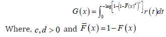
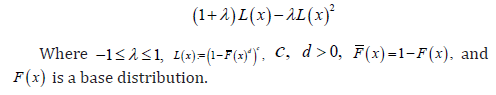
Remark 1.5. Note that if we set 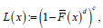 where ,0cd> and ()()1,FxFx=− then ()Lx gives the CDF of the exponentiated generalized class of distributions [8]

Further developments

In this section, inspired by quantile generated probability distributions and the T transmuted X family of distributions [6,9], we propose some new extensions of the exponentiated generalized (EG) T-X family of distributions. We give the CDF of these new class of distributions, only in integral form. However, the CDF and PDF can be obtained explicitly by applying Theorem 2.2 and Theorem 2.3, respectively.

The TqX− family of distributions

Definition 2.1. Let V be any function such that the following holds:

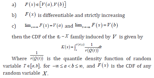
Theorem 2.2. The CDF of the TqX− family induced by V is given by ()()()KxQVFx

Proof. Follows from the previous definition and noting that 

Theorem 2.3. The PDF of the TqX− family induced by V is given

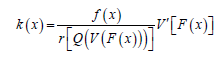
Proof. ,k=K′,  F′=f and K is given by Theorem 2.2

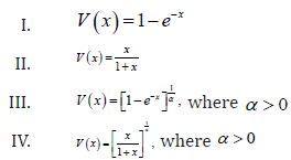
Remark 2.4. When the support of T is [),,a∞ where 0,a≥ we can take V as follows

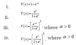
Remark 2.5. When the support of T is (),,−∞∞we can take V as follows

Definition 2.6. A random variable W (say) is said to be transmuted exponentiated generalized

distributed if the CDF is given by

Some EG Tq transmuted X family of distributions

In what follows we assume the random variable T has PDF ()rt and quantile function ().Qt We also assume the random variable X has transmuted CDF

Families of EG Tq-transmuted X distributions of type I

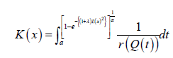
The CDF has the following integral representation for α>0 and a≥0

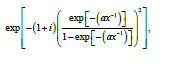
Families of EG Tq transmuted X distributions of type II

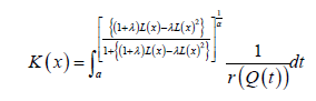
The CDF has the following integral representation for α>0 and a≥0

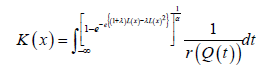
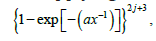
Families of EG Tq transmuted X distributions of Type III

The CDF has the following integral representation for 0α>

To Know More About Biostatistics and Biometrics Open Access Journal  Please click on: https://juniperpublishers.com/bboaj/index.php

 

To Know More About Open Access Journals Please click on: ttps://juniperpublishers.com/index.php

Algebraic-Probabilistic Methods and Grobner Bases for Modeling the Brain Activity-Juniper Publishers

Biostatistics and Biometrics Open Access Journal 

Building accurate representation of the world is one of the basic functions of the brain. In order to better understand its functioning, in [1-4] the authors develop and study theoretically the neural codes model, whose main purpose is to describe stereotyped stimulus response maps of the brain activity. We suggest a modification of this model, which has a potential to be more suited for practical applications. It is worth mentioning that the modified model we suggest requires tools from various parts of mathematics, not just algebra as is the case for the original model.

First, we briefly outline the original neural codes model as described in [1-4]. To each neuron v in the brain corresponds a convex subset the collection of the states (e.g., spatial position) in which the neuron v activates. Now for each point x in , we have a vector

Note that vectors. The (obviously finite) collection

of 0–1 vectors is called the neural code and is the object of study in [1-3]. The method used in [1-3], is purely algebraic. Namely, one considers the collection t_v of commuting independent variables (one per each neuron) and the algebra of polynomials in these variables over the 2-element field 2.F To each aC∈ we assign the ‘pseudomonomial’ and generate the ideal CI by all .af It is shown in [1-4] that knowing the ideal ,CI one can recover C (no information is lost). Then we have the toolbox of combinatorial algebra at our disposal: one can study the ideals generated by collections of pseudomonomials and gain information about neural codes. One of the main tools applied is the Grobner basis technique, as it is classically used in commutative algebra [5,6].

There is one obvious problem though: the enormous number of generators of the algebra A. Grobner bases are sometimes nice and effective but only if the presentation of the ideal is small enough. The punch-line is that the above model is easy to deal with by means of appropriate software for toy illustrative problems, but once we approach any real life situation, not even a supercomputer will ever cope [7,8].

We suggest the following modification of the neural codes model. Rather than dealing with individual neurons, we suggest to consider their clusters. The number and the size of clusters can be adjusted when dealing with each practical situation. Instead of the 0–1 outcome of the interaction with the environment, we measure the total activity p of the cluster: the ratio of the number of active neurons to the total number of neurons in the cluster. Thus p is a real number between 0 and 1 with p=0 standing for total inactivity and 1 for the entire cluster being ’on fire’. The number p can be viewed as the probability of a neuron in the cluster to activate. As a result, the convex sets U are replaced by functions

with x_c(x) standing for the probability of a neuron in the cluster c to activate in the estate .x There are various ways to analyze such a model. We suggest the following approaches.

Approach 1

Geometric

Unlike for the neural code, for which all vectors are far apart from each other, the set

is a genuine geometric object, where C is the set of all clusters under consideration and M is their number. Depending on the assumptions (or natural properties) on the functions (),cux the set ˆ,C can have different geometric properties. One may look for extremal and corner points of ˆ,Cstudy smooth curves in ˆC etc. Note that if one interprets ˆC as a CW-complex, then there is the natural b task of determining its homologies. Although this particular task is insurmountable in most cases, there is a hope in the form of the emerging method of persistence homology being developed for the study of big data. We would mention here also our results on exact methods of calculating homology, which fall into the frame of persistent homology [9,10].

Approach 2

Stochastic

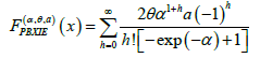
After appropriate normalization, each ()cux provides a probability distribution Now one can deal with the model by studying the random vector 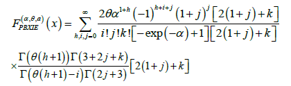which yields a whole host of possibilities, not to mention the ability to use the vast toolbox of probability theory. One interesting and potentially very important aspect that can be captured in this way is the correlation between the response of the clusters. This can be viewed as the study of the relations between different parts of the brain from the probabilistic point of view.

Approach 3

Probabilistic algebra

One can pursue the same strategy as in [1-3], where instead of a single ideal in the algebra of polynomials we shall have a ’random ideal’: a family of ideals with a probability distribution on it. Such an object can be studied using the same old methods of combinatorial algebra including the Grobner basis technique. The answers are going to come with the randomness embedded in them. For instance if we use the Grobner basis to compute the Hilbert series of the quotient by our ideal, we end up with a probability distribution on the set of formal power series instead of a single series. Note however that such distributions tend to be discrete rather than continuous even when the starting distribution was a continuous one. The advantage of this approach is in the fact that the number of generators is reduced.

To Know More About https://juniperpublishers.com/bboaj/index.php Please click on:

https://juniperpublishers.com/bboaj/index.php

 

To Know More About Open Access Journals Please click on: ttps://juniperpublishers.com/index.php