In this paper, the general behaviour of the marine
circulation (sea currents) and the resulting patterns caused by wind
action in the central part of the South Euboean Gulf is studied using a
three-dimensional hydrodynamic model (ELCOM). The work was part of a
study effort to exploit the fresh water jets that spring from the bottom
of the sea, off the port of Eretria (these underwater karstic springs
in the sea are called anavalos in Greek). The specific objectives were
to determine the shape of the depth-averaged currents resulting from
typical wind conditions and to estimate the typical time of adaptation
of currents to changes in wind conditions. The South Euboean Gulf is a
relatively narrow strait formed between Attica and the southernmost part
of the NE coast of Central Greece, with only its central part having a
considerable width, and extends for about 55 nautical miles from
southeast to northwest. For the bathymetry a variable grid was used and
the model was put to run simulations for each of the eight primary wind
directions, for a time period of three consecutive days and then pause
abruptly. The simulation period extended to seven days so as to consider
the times of adaptation. No stratification was considered. The results
seem very plausible and indeed are confirmed by dimensional analysis
that is included in this paper as an appendix.
Keywords: Wind induced sea currents; South Euboean Gulf; Greece; ELCOM model
The Euboean Gulf has been a subject of scientific
inquiry from the days of the ancients Greeks, due to the very strong
tidal effect that characterizes the strait of Euripus, near the city of
Chalkis. The strait is subject to strong tidal currents which reverse
direction approximately four times a day. Although tidal flows are very
weak in the Eastern Mediterranean, this strait is an exception. Amongst
the early scholars who studied the phenomenon we find Eratosthenes,
Pitheas, Posidonios, Stravon and Senekas. There is even a tradition that
Aristotle committed suicide by falling into the waters of Euripus,
because he could not solve the problem, saying the famous "Since thou
did not send Euripon to Aristotle, thou sent Aristotle to Euripus". This
is a myth of course, because Aristotle died in Chalkis, but he died a
natural death. The Gulf has been the subject of a number of studies also
from the early 20th century. Forel, the ‘father’ of
Limnology, was one of the first to suggest an explanation, but a more
complete analysis was presented by Aiginitis, director of the Athens
Observatory, who published his conclusions in 1929.
The shape of the Gulf, and especially its southern
part, south of Chalkis, being effectively an enclosed sea water body
with very specific boundary conditions to its Northern end, lends itself
to hydrodynamic modelling. The first hydrodynamic model for the whole
of the Gulf (both its Northern and its Southern part) was constructed by
Livieratos, while Tsimplis applied two models, a low resolution one for
the propagation of tidal waves in the northern and southern Euboean
Gulf and a high resolution one, focused on the Gulf’s Straits.
Tsirogiannis et al. simulated the whole of the Euboean Gulf using the
ELCOM model with important findings [1].
It is important to understand the physical processes
and mean circulation patterns since they provide an indication of
transport pathways of nutrients, contaminants and sediment (suspended
particles). To this end, 3‐D coastal ocean models have been developed by
various researchers and Universities, like for instance Princeton Ocean
Model (POM), which is considered one of the first. One such model is
ELCOM that solves the hydrodynamic and the continuity equations assuming
hydrostatic conditions and the Boussinesq assumptions. ELCOM (Estuary,
Lake and Coastal Ocean Model) [2] has been developed by CRW (Center for
Water Research, University of Western Australia), and has been used
extensively over the last 15 years in simulating marine and coastal
ocean environments, lakes [3-5], river plume dynamics [6] and even
stabilization ponds systems [7]. Modeled and simulated processes include
baroclinic and barotropic responses, rotational effects, tidal forcing,
wind stress, surface thermal forcing, inflows, outflows, and transport
of salt, heat and passive scalars [7]. It is worth noting that ELCOM
usually requires minor calibration adjustments, since the variation of
most of its parameters is well defined by the conservation equations of
mass, momentum and energy containing few adjustable coefficients, unlike
its coupled model CAEDYM, dedicated to water quality simulation, that
appears more sensitive to field data [5].
This study can be thought of as a numerical
experiment or investigation, in the sense that no measured/observed
field data were used for the simulations or the validation. The
meteorological forcing was represented by a seasonal average for the
seven days that each of the eight simulations was performed-one for
every wind direction. The purpose was to determine the shape and
magnitude not only of the surface currents, but also the bottom and
depth-averaged circulation resulting from typical wind conditions.
Study Area
The South Euboean Gulf is formed between the eastern
coast of Attica (southwards) and the southernmost part of the NE coast
of Central Greece (northwards) which form its south-western shores and
the southernmost part of the SW coast of the island of Evia which form
its NW shores. This rather narrow and elongated sea area extends for
about 55 nautical miles from southeast to northwest and is divided into
three distinct parts: The Gulf of Petalia or outer part, the central
part and the innermost point of South Euboean which in turn consists of
the inner (northwest) part, the Strait of Diaylos and the South Port of
Chalkida [8].
The central part of the South Euboean Gulf (Figure
1), which is the study area, has the southeastern boundary of Akra
(=cape) Paliofanaro of the Kavalliani Island, the southwestern boundary
of Akra Agia Marina and the northwestern boundary of Akra Avlidos, about
24 miles northwest of Akra Agia Marina, while the northeastern boundary
is Akra Bourtzi, which is located at the same distance northwest of
Akra Paliofanaro. This section extends for about 25 miles (46.3 km) from
SE to NW and its width, around its middle, is 8 miles (14.8 km). The
southern entrance (Kavaliani) of the central part is 1.4 miles (2.59 km)
wide, while the northern entrance (Avlida) is 3/10 of a mile (0.55 km)
wide and is the narrowest point of the strait of the same name
(Avlida-Bourtzi). The extent of the sea area of the central part is
about 460 km2 and the perimeter is roughly 160 km.
The sea depths at the southern entrance are about 70m
in the middle of the distance between Isl. Kavaliani and Akra Agia
Marina, while along the axis of the Avlida Strait the depths range from 8
to 14 m. The bathymetry of the bay reveals the existence of a steep
slope in the direction west to east where a difference in depth of about
25 m is observed over a length of about 10 km (from the middle of the
distance between Eretria and Amarynthos to the coast of Amarynthos).
This slope can be said to divide the bay into a deep eastern part (east
of Amarynthos) with an average depth of 53m, and a shallow western part
(west of Eretria) with an average depth of 23m. The depths in the cove
(inner part and South Port of Chalkis) are much shallower with a maximum
depth of 10 m.
The prevailing winds according to the wind data of
the Chalkida meteorological station are the North (23.4%), the Northeast
(21.7%) and the Northwest (17.9%). The other winds occur with
relatively low frequency (5÷7%), except for the West winds which occur
relatively more frequently than the others (8.1%) [8]. Cloudiness occurs
5% of the time
ELCOM model and set-up
For the numerical simulation, as earlier mentioned,
the ELCOM (Estuary, Lake and Coastal Ocean Model) model was used, a 3D
finite-difference model suitable for simulations in lakes and enclosed
water bodies. The main equations are the Reynolds averaged Navier-Stokes
(RANS) equations using the Coriolis term, following the Boussinesq
approximation and ignoring non-hydrostatic pressure terms. For the
turbulence, as far as the horizontal is concerned, a constant eddy
viscosity coefficient is used, while for the vertical the coefficient is
obtained as a function of a local Richardson number. The density is
calculated as a function of temperature and salinity according to the
UNESCO equation [2].
The bathymetry was derived from digitizing the map of
the Hydrographic Service of the Navy. The horizontal resolution was
200x200 m in the largest part of the field, while in parts of the field
cells of other dimensions were used (non-uniform grid) in order to
represent dimensions smaller than 200 m (such as the Euripus Strait).
The total number of surface cells was 11,565. The following
surface-to-bottom resolution was used for the vertical: 0.5 +0.5 +0.7
+0.8 +1.3 +1.7 +2 +2.5 +2.5 +2.5 +5 +7 +8 +10 +10 +10 +10 = 75m. The
total number of computational cells was 162,565. A constant and uniform
sea temperature of 17ºC (late autumn - spring), and a constant wind
speed of 7 m s-1 (4 Beufort) was assumed. In the northern and
southern boundaries of the computational domain, an “open” boundary
condition was applied, which passively allowed the water inflow to, or
outflow from each cell, according to the corresponding flow needs.
The time step was 30 sec. and the duration of the
simulation was 7 days for each of the eight winds. The wind blew
continuously for the first 3 days and stopped abruptly at the beginning
of the fourth day. Both the dimensional analysis and the results of the
simulations showed that this time period was sufficient for the flows to
stabilize at the end of the third day (in fact in a much shorter time).
The inertial oscillations that followed the wind cessation, however,
generally did not seem to fully damp out over the next 4 days. For the
visualization of the results, the model allows the creation of
“curtains” i.e. sections of the water body along given lines, as well as
three types of plan views or “sheets”: the surface layer (top), the
bottom layer (bottom) and finally the average layer (average), which is
the depth-integrated result of the parameter of interest. We used two
perpendicular 'curtains' (Figure 1) at the intersection of which the
position of the Eretria’s anavalos is roughly located. These curtains
are a) Eretria - Oropos and b) Avlida - Aliveri. It should be emphasized
here, for the sake of understanding the diagrams that follow, that the
speed U increases downwards, while the speed V increases to the right.
Thus, V is perpendicular to the curtain of Eretria (with positive values
meaning flow towards Aliveri), while U is perpendicular to the curtain
of Avlida (with positive values meaning flow towards Oropos). Finally, a
tracer (Tracer_3, Figure 1) at the intersection of the two curtains was
used to visualize circulation at this location.

Below we will describe the actual three-dimensional
circulation patterns resulting from the wind blowing for a long time
from a given direction. We are going to consider winds in pairs in order
to avoid confusion from the many cases.
North - Northeastern wind
On the surface, the Northern wind breeze causes
'gusts', i.e. areas of confluence of relatively strong currents in a SW
direction, while offshore, i.e. towards the Gulf of Aliveri, they take a
more Western direction, as the Figure 2 shows. The northeast wind blast
causes stronger currents with a westerly direction. A strong 'gust'
passes off Eretria, with speeds up to 1m/s. However, it should be
mentioned that of the 8 winds simulated, NE appeared unstable, i.e. the
equilibrium state at the end of the adjustment time was not evident.
The circulation on the seabed created by the Northern
wind is generally directed E and NE except for the bay of Chalkoutsi
where the seabed flows 'turn' to NW (Figure 3). The resulting average
circulation, as shown in Figure 3, is a cyclonic gyre with higher
average speeds on the southern coast (Oropos and Chalkoutsi). We can
observe this pattern also in the Eretria curtain with lines of equal V
velocities in Figure 4.
As one can see in Figure 4, the transport to Avlida
takes place on the surface, while deeper there is transport to Oropos.
Positive velocities - towards Aliveri - are found throughout the central
part at depths below 10 m and mainly in the deeper parts of Eretria.
Velocities here reach and exceed 5 cm/s. Figure 4 on the right is more
difficult to read as the U velocity is parallel to the axis of the plot.
However, a surface layer of about 5 m thickness with transport towards
the Oropos and velocities at the surface of ~20 cm/s is shown here,
while deeper in the Oropos a return current with velocities of ~5 cm/s
is shown which occurs at a depth of 6 to 13 m. The total transport that
takes place in the region can also be visualized using the tracer, and
is shown in Figure 5. As we can see, the current generated at the
surface is 45 degrees to the right of the wind, while at the bottom it
is 90 degrees to the left. The average transport is almost similar to
the bottom transport indicating that the main transport occurs with the
bottom Ekman layer rather than the surface layer. The shape of the
spiral is shown in Figure 5 below which is the Avlida-Aliveri curtain.


Western – Northwestern wind
On the surface, the westerly wind creates strong
surface currents along the southern coasts (Dilesi - Chalkoutsi - Oropos
- Ag. Marina). The NW wind breeze creates a nearly homogeneous surface
velocity field with a N to S direction (Figure 6).
On the bottom, with a westerly wind, we have a
reverse flow to the W and NW in the centre of the bay and near Eretria,
while on the southern coast we have the same flow as the surface flow.
The average transport occurs on the North and South coasts towards E and
SE with a small return flow in the centre of the bay. Overtopping is
observed on the W oriented coasts. With a NW wind, the velocities in the
bottom layer shift to the north. The free surface level is lowered in
the interior of the bay. The surface speed of the current is at 45
degrees to the right of the wind. The bottom velocity as well as the
average is again at 90 degrees to the left of the wind.

The NW wind circulation on the surface is therefore
towards Oropos, while in deeper parts of the bay is towards Eretria.
This is illustrated in Figure 7 where in the surface layer of about 10 m
thickness the transport is towards Oropos, while below this depth there
is a weak flow in the opposite direction, with higher velocities
~5cm/s, in the layer from 10 to 20 m depth, and mainly within the
shallow part of the bay.
Southern - Southwestern wind
At the surface the southern wind creates currents
with a Northeastern direction. The Southwestern wind creates strong
currents on the northern but mainly on the southern coast of the bay.
To the south, there is a set-up on the north coast
with a SW orientation. The bottom circulation is mainly to the north
coast in an easterly direction and on the south coast to a westerly
direction. The average circulation is very similar to the bottom
circulation. With Southwestern wind there is there is a set-up on the
coast with a western orientation (Buffalo Bay). On the bottom we have a
reverse direction mainly in the centre of the bay while on the North and
South coasts we have an Eastern direction. The average circulation is
again similar to the bottom circulation.
Eastern - Southeastern wind
At the surface, the easterly wind creates straight
currents along the Northern shores in W and NW direction. The southeast
wind creates a nearly uniform velocity field on the surface in a
northerly direction. The Eastern wind creates currents on the North
coast of approximately the same direction as the surface currents. There
is a return to the East parallel to the south coast. With a
southeasterly wind the bottom circulation is the reverse of the surface
circulation, i.e. to the south. On the south coast it turns to the west.
This modeling study aimed at recognizing and
quantifying the patterns of the sea currents induced by wind forcing and
the resulting circulation. 3D simulations with ELCOM provide a host of
possibilities for physical investigation in simulating both real time,
short-term, complex marine processes but also in simulating medium and
long term processes. Although the main processes can be hypothesized
from theory and accumulated experience, the quantification and magnitude
of the phenomena is greatly enabled by the application of the 3D
hydrodynamic and thermodynamic models. In general, the application of
such models in various coastal and estuary environments for a variety of
purposes has been proven to be not only plausible but accurate as well
[9]. The focus each time depends on the purpose and scope of the
research, but there always seem to be some unpredicted -or unthought of-
findings.


One such finding of the current study is that all 3
Northern winds, that prevail in the study area occurring more than 63%
of the time, and with higher intensities, induce a transport of finer
bottom sediment from the shores of Attica to the shallower western part
of the Gulf, and partially to the across shores of Evia on a never
stopping ‘conveyor belt’. The basin bed layer of the southern Euboean
Gulf consists of Holocene sediments that might extend to a thickness of
14 m, while the sea bottom is dominated by mud except for the shallow
coastal areas, where the sand may reach up to 50% of its overall
consistency [1]. According to published maps regarding the state of the
shores in Greece the western shores of Euboea appear stable, contrary to
the opposite shores of Attica that experience erosion. This finding
remains to be studied further and proven, or unproven, but it
exemplifies the capacity of the 3D hydrodynamic models to study and
model marine sediment transport issues, albeit indirectly.
In all cases the average transport due to the
generated currents is at 90º to the left of the wind vector, i.e. that
of the Ekman bottom layer. The prevailing northern winds induce a gyre
that carries finer bottom sediment from the shores of East Attica to the
shallower part of the Gulf, towards Avlida, and partly to the shores of
Euboea. The generated currents at the surface have velocities that vary
depending on the wind direction and range from 20÷60 cm/s. At the
bottom, compensatory currents develop with velocities of up to 5 cm/s.
The adaptation of the sea circulation (the equilibrium state) to the
surface due to the wind blast occurs in about 18-24 hours from the
beginning of the episode. The bottom circulation seems to reach
equilibrium earlier, at 10-14 hours. The cessation of the wind is
followed by inertial oscillations that fully decay in about 5 days. The
latter results are further supported by the analysis in the appendix.
Although numerical model simulation can extend and
quantify our knowledge of the hydrodynamics of a marine region, the main
physical processes must be known in advance. One of the reasons why
this pre-estimation is necessary is the selection and tuning of the
model. We will therefore attempt below to make an assessment of the main
scales, both temporal and spatial, that characterize the marine
circulation phenomena in the central part of the South Euboean Gulf.
The Coriolis effect
The Coriolis 'force', as we know, is the result of
the rotation of the earth and causes the movements to be deflected to
the right (left) in the northern (southern) hemisphere. We can weight
this effect using the inertial radius rc and the inertial period Tcor.
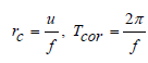
where f is the Coriolis parameter (f = 2Ωsinφ, Ω is the rotational speed of the Earth, Ω ≈ 7.2921*10-5 rad s-1 and φ is the latitude of the place, f = 8.9789*10-5 for latitude φ = 38º) and u (ms-1) is the speed of motion.
If the event in question (current motion, long-wave passage, etc.) is of a time period sufficiently shorter than Tcor,
then there is 'not enough time' to deflect the direction of motion,
while if the size of the basin is sufficiently smaller than rc
then the Coriolis force 'does not have enough space' to turn the
velocity vector. In the case under consideration we have the following
magnitudes:
From the above table (Table 1) we conclude that for speeds such as those of sea currents (~0.2 m s-1) there will be a significant effect of the Coriolis force, as the width of the basin (Lwidth ~ 15 km) is much larger than rc, while for speeds such as that of a long wave (u = [gh]1/2 ~ 20 ms-1) there is no Coriolis effect.
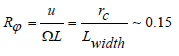
The Rossby number, Rφ, expresses
the ratio of the translational accelerations to the Coriolis
accelerations, (which should be of the order of 0.1 or less for there to
be a significant Coriolis effect) and the appropriate length, L, is the
width Lwidth of the basin

Ekman Currents
The estimation of the velocities and shape of sea
currents caused by the wind blast can be done by Ekman's (1905) theory.
This theory describes the currents in the upper layers of the sea in
equilibrium under the influence of the wind shear stress and friction of
the water layers during their movement, the Coriolis force, and the
local pressure gradient (the slope of the water surface). The amount of
motion is transmitted from the surface to the deeper layers through
vertical turbulent mixing (eddy viscosity) with a constant (according to
Ekman) coefficient Kz.
As is well known, the direction of the surface
current forms a 45 degree angle to the right of the wind direction (in
the northern hemisphere) and its speed (which at the surface is UE) decreases exponentially with depth. At depth z = hE
the current direction turns in the opposite direction to that at the
surface and the water velocity at this depth has decreased by exp(-π), at a rate of about 4.3% relative to the velocity at the surface UE.
This form is called the Ekman spiral. The main transport of water due to the current occurs at a depth z = hE
/2 and is at an angle of 90 degrees to the right of the wind direction.
Before establishing a free surface slope and at times shorter than the
adjustment times (which we will discuss later) the sizes mentioned above
are given by the following formula:
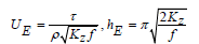
Where τ is the wind stress (Pa), ρ is the density of seawater (= 1027 kg m-3), Kz (m2 s-1)
is the constant eddy viscocity coefficient. The wind tension τ depends
on a coefficient C (Ekman used the value C = 0.0026), the air density ρa, ρa = 1.25 kg m-3, and U10 (m s-1) the air speed at a height of 10 m above the sea surface.

So, for a typical value of Kz = 10-3 m2 s-1
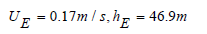
From the literature, Ekman used the following formulas
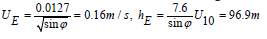
for UE10 = 10m/s
Observations and measurements since then have finally
given a surface velocity equal to half that predicted by Ekman, while
the thickness of the layer was measured in very good agreement with its
predicted value. At the bottom, if there is some motion, an Ekman layer
will also occur in reverse order to the surface layer. This layer is
called the Ekman bottom spiral.
Time scale of current adaptation
Due to the inertia of the water the wind will start
to shape the surface currents with some delay. The Coriolis effect will
become noticeable after t > 0.25/f ~ 46 min. The adaptation period as
a whole can be approximated as

where H may be the average depth of the basin assuming that the basin is fully mixed. If we assume H = 44m and Kz = 10-3 m2 s-1 we have T = 2.5 days approximately, while with Kz = 10-4 m2 s-1 we have T = 7.8 days approximately.
Stream structure in equilibrium
In closed basins the prolonged wind blow will create
an elevation of the water surface in the downwind direction (wind
set-up). Since this will create a pressure gradient, it will also cause a
compensatory flow (return flow) which takes place in the deeper layers
of the basin. This circulation is complex and depends on the topography
of the seabed, possible stratification, wind conditions, etc. This flow
will be generated within a long-wave travel time, i.e. within about 10
minutes for a distance such as that between Eretria and Oropos (L/u
=7500/17=7.3 min).
An estimate of the level difference Δh in the direction Eretria - Oropos is
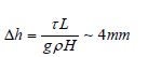
with H=30m, L=7500 m and τ = 0.162 Pa.
For an estimate of the velocity resulting from this level difference
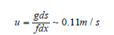
which is however considered to overestimate the actual velocity since it does not take into account the friction on the bottom.
Inertial Oscillations
If the wind suddenly deafens or changes direction
then the process of adjusting the water flows under the influence of the
earth's rotation to a new equilibrium state will be accompanied by
oscillations around this new equilibrium position. These inertial
oscillations have a characteristic period Tcor (~19h). The
damping rate of these oscillations depends on their inertial period. The
time scale of the adjustment of the currents to a new pressure gradient
is t >> 1/f ~ 3 h. A good approximation is t~3÷5 Tcor,
i.e. t ~ 2.3 to 4 days. For an estimate of the minimum adaptation time
we can consider half the period of the single-node oscillation (seiche,
see below).
It should be stressed that in case the basin depth is
greater than hE a distinction between the two time scales should be
made in order to adapt the currents to the surface layer. These time
scales correspond to
a) Ekman adjustment due to Coriolis and frictional stresses in the Ekman layer
b) Inertial motion due to Coriolis and pressure gradients
It should also be mentioned that in case the wind
stops we will have the creation of standing waves (seiches) in the basin
(if it is closed). The period of these standing waves is given by
Merian's formula:

where n is the number of nodes in the oscillation. For a single-node (n=1) oscillation we have Th
= 12.6 min for the route Eretria - Oropos.
To Know More About Juniper Online Journal Material Science Please click on:
https://juniperpublishers.com/jojms/index.php
For more Open Access Journals in Juniper Publishers please click on:
https://juniperpublishers.com/index.php


