Friday, May 24, 2024

Intramural and Adapted-Germ Cell Neoplasia in Situ - Juniper Publishers

 Cancer Therapy & Oncology - Juniper Publishers


Abstract

Germ cell neoplasia in situ emerges as a precursor lesion configuring type II germ cell tumors as testicular seminoma or post-pubertal non-seminoma Tous testicular germ cell tumors. Lesion is comprised of neoplastic gonocyte-like cells, latent totipotent or naive germ cells with developmental potential situated within ‘spermatogonia niche’ of seminiferous tubules. Germ cell neoplasia in situ delineates an increased incidence with conditions such as uncorrected cryptorchidism, ambiguous genitalia, infertility or preceding history of post-pubertal germ cell tumor within contralateral testis. Neoplasm demonstrates aneuploidy or polypoid genotype with additional chromosomal gains as isochromosome 12p upon commencement of neoplastic invasion. Neoplastic cells appear enlarged, atypical, gonocyte-like and are incorporated with abundant, clear cytoplasm, enlarged, hyperchromatic nuclei, coarse nuclear chromatin, angulated cellular margins and prominent nucleoli.

Keywords: Precursor lesion; Primordial germ cells; Aneuploidy; Bilateral microlithiasis; Chemotherapy

Abbreviations: WHO: World Health Organization; GCNIS: Germ Cell Neoplasia in Situ; UNL: Upper Normal Limit; LDH: Lactic Dehydrogenase; FISH: Fluorescent in Situ Hybridization; SNP: Single Nucleotide Polymorphism; PLAP: Placental Alkaline Phosphatase; AFP: α fetoprotein

Introduction

Germ cell neoplasia in situ is a commonly discerned precursor lesion configuring type II germ cell tumors as testicular seminoma or post-pubertal non-seminomatous testicular germ cell tumors. Lesion is comprised of neoplastic gonocyte-like cells and latent totipotent or naive germ cells with developmental potential which are situated within ‘spermatogonial niche’ of seminiferous tubules. As per current World Health Organization (WHO) classification, neoplasm is designated as germ cell neoplasia in situ and represents as a precursor for a subset of adult germ cell tumors. Alternative terminology as intra-tubular germ cell neoplasia, intra-tubular germ cell neoplasia unclassified subtype, carcinoma in situ testis or malignant germ cells is not recommended. Appropriate discernment of germ cell neoplasia in situ may be challenging, especially in pediatric subjects or individuals demonstrating infantile or pre-pubertal testis on account of morphological concurrence and immunohistochemistry concordant with normal or delayed maturation of testis. Surgical sampling of a testicle from subjects incriminated with extra-gonadal germ cell tumor may represent with ‘burnt out’ germ cell tumor.

Germ cell neoplasia in situ expounds an increased incidence with associated conditions such as uncorrected cryptorchidism, ambiguous genitalia, infertility, or preceding history of post-pubertal germ cell tumor within contralateral testis. Frequently, lesion is accompanied by aneuploidy although lack of isochromosome 12p appears within invasive adult germ cell tumours [1,2]. Molecular assay of neoplastic cells demonstrates aneuploidy or a polypoid genotype with additional chromosomal gains occurring upon commencement of neoplastic invasion, as enunciated with isochromosome 12p discerned within invasive disease and absent within germ cell neoplasia in situ [1,2]. Frequently, germ cell neoplasia in situ arises within testicular seminiferous tubules incriminated with post-pubertal germ cell tumours and occasionally represents as a residual manifestation or ‘burnt out’ germ cell tumour [2,3]. Germ cell neoplasia in situ is posited to arise from incompletely differentiated primordial germ cells which expound whole genome duplication events with subsequent repetitive loss of chromosomal arms or entire chromosomes. Therefore, an aneuploidy within the neoplastic configuration ensues with subsequent emergence of additional chromosomal mutations within a subset of tumefaction as genetic mutations within KIT gene or KRAS gene [2,3].

Preliminary genomic mutations within KIT gene following genome duplication may engender a subset of testicular seminoma comprehensively delineating genomic hypomethylation. Besides, differentiation into diverse histological subtypes is absent. Germ cell neoplasia in situ is postulated to manifest as a ubiquitous precursor of type II germ cell tumours which represent ~95% of germ cell tumours arising within post-pubertal males as testicular seminoma, embryonal carcinoma, choriocarcinoma, testicular teratoma or yolk sac tumour [2,3]. Overexpression of embryonic transcription factors may elevate cellular proliferation and abolish apoptosis. Germ cell neoplasia in situ is comprehensively encountered within testicular seminiferous tubules incriminated with adult germ cell tumours. Occasionally, contralateral testis may exhibit foci of germ cell neoplasia in situ. Additionally, lesion may concur as a residual feature with ‘burnt out’ adult germ cell tumour [3,4]. Upon microscopy, neoplastic cells appear confined to basement membrane of seminiferous tubules and configure a designated ‘spermatogonial niche’ [3,4]. Neoplastic cells appear enlarged, atypical and gonocyte-like and are incorporated with abundant, clear cytoplasm, enlarged, hyperchromatic nuclei, coarse nuclear chromatin, angulated cellular margins and prominent nucleoli, reminiscent of seminoma cells. Tumour cell nuclei appear up to 11 μ metres in diameter. Frequently, incriminated seminiferous tubules delineate a thickened basement membrane, peritubular hyalinization and lack of spermatogenic maturation. Tumefaction demonstrates a ‘pagetoid’ pattern of neoplastic dissemination into rete testis or a plane between epithelium layering rete testis and basement membrane [3,4] (Figures 1 & 2).

TNM staging of carcinoma testis [3,4]

Primary tumour

i. TX Primary tumour cannot be assessed.

ii. Tis Germ cell neoplasia in situ (GCNIS).

iii. T0 No evidence of primary tumour within the testis.

iv. T1 Primary tumour confined to testis and rete testis.

Vascular or lymphatic infiltration is absent. Tunica albuginea is invaded. Tumour invasion into tunica vaginalis is absent.

Pure seminoma is subdivided as:

i. ~T1a Tumour magnitude < 3 centimetres.

ii. ~T1b Tumour magnitude ≥ 3 centimetres.

iii. T2 Tumour confined to testis, rete testis and extends into ≥ one components of testis as blood vessels, lymphatics, epididymis, adipose tissue confined to hilar soft tissue adjacent to epididymis or tunica vaginalis.

iv. T3 Tumour extends into spermatic cord.

v. T4 Tumour extends into scrotum.

Regional lymph nodes

Clinical staging of regional lymph nodes is assessed with imaging techniques such as computerized tomography(cN).

Pathological staging of regional lymph nodes is assessed with dissection of regional, retroperitoneal, para-aortic, peri-aortic, inter-aortocaval, paracaval, pre-aortic, precaval, retro-aortic and retrocaval lymph nodes(pN).

i. NX Regional lymph nodes cannot be assessed.

ii. N0 Regional lymph node metastasis absent.

iii. N1 Regional lymph node metastasis confined to one to five retroperitoneal lymph nodes with magnitude < 2 centimeters.

iv. N2 Regional lymph node metastasis into minimally a singular enlarged lymph node or lymph node mass >2 centimeter and <5-centimetre diameter OR metastasis into >5 regional lymph nodes <5-centimeter diameter OR metastasis into minimally a singular lymph node between 2 centimeter and 5-centimeter diameter.

v. N3 Regional lymph node metastasis into minimally a singular enlarged retroperitoneal lymph node or lymph node mass > 5-centimeter magnitude OR metastasis into minimally a singular enlarged lymph node or lymph node mass > 5-centimeter diameter.

Distant Metastasis

i. MX Distant metastasis cannot be assessed.

ii. M0 Distant metastasis into distant lymph nodes or various organs absent.

iii. M1 Distant metastasis into:

a. ~M1a Metastasis into pulmonary parenchyma or distant lymph nodes as pelvic, thoracic, supraclavicular or visceral lymph nodes apart from retroperitoneal lymph nodes.

b. ~M1b Distant metastasis into viscera as hepatic parenchyma, skeletal system or brain. Pulmonary parenchyma may or may not be incriminated.

Serum Tumour Markers

i. SX Serum tumour marker levels unavailable.

ii. S0 Serum tumour marker levels appear normal.

iii. S1 Minimally a singular tumour marker level exceeds normal range as

a. ~lactic dehydrogenase (LDH) <1.5 times upper normal limit (ULN)

b. ~βHCG < 5,000 mIu/mL.

c. ~alpha fetoprotein (AFP) <1,000 ng/mL.

iv. S2 Minimally a singular tumour marker appears substantially above normal range as.

a. ~lactic dehydrogenase (LDH) between 1.5 times to 10 times upper normal limit (ULN).

b. ~βHCG between 5,000 to 50,000 mIu/mL.

c. ~alpha fetoprotein (AFP) between 1,000 to 10,000 ng/ mL.

v. S3 Minimally ≥ one or more tumour markers are significantly elevated.

a. ~lactic dehydrogenase (LDH) > 10 times upper normal limit (ULN).

b. ~βHCG > 50,000 mIu/mL

c. ~alpha fetoprotein (AFP)> 10,000 ng/mL

Discussion

Tumour cells appear immune reactive to OCT3/4, SALL4, podoplanin or D2-40, SOX17, NANOG, LIN28A, AP2 gamma, placental alkaline phosphatase (PLAP) and c-KIT or CD117. Tumor cells appear immune non-reactive to α-inhibin, SF1, Wilm’s tumor 1(WT1) antigen, pan-cytokeratin AE1/AE3, CD30, SOX2, α fetoprotein (AFP) or glycpican 3 [5,6]. Germ cell neoplasia in situ requires segregation from neoplasms such as infantile or prepubertal testis with gonocytes or normal or delayed testicular maturation, intratubular seminoma or seminoma with microinvasion [5,6]. Fluorescent in situ hybridization (FISH), single nucleotide polymorphism (SNP) array or genetic karyotyping may be beneficially adopted to detect aneuploidy or absence of isochromosome 12p. Germ cell neoplasia in situ can be appropriately ascertained with precise histological examination of surgical tissue samples as testicular biopsy or orchiectomy. Alternatively, tissue sampling of contralateral testis incriminated with adult germ cell tumor may be beneficially adopted. Neoplasm is devoid of specific serum biomarkers or pertinent features in imaging. Upon ultrasonography of subjects demonstrating infertility, unilateral or bilateral microlithiasis may be discerned, a feature which is associated with enhanced incidence of germ cell neoplasia in situ [5,6].

Surgical tissue sampling of testis may be adopted in subjects delineating microlithiasis along with minimally a singular, concurrent condition as uncorrected cryptorchidism, ambiguous genitalia, infertility or preceding history of post-pubertal germ cell tumour within contralateral testis [5,6]. Germ cell neoplasia in situ can be appropriately treated with orchiectomy. Besides, extensive surveillance is recommended to evaluate neoplastic progression. Employment of adjuvant chemotherapy appears non concurrent with decimation of risk of disease progression. Low dose radiotherapy may be contemplated for alleviating germ cell neoplasia in situ within contralateral testis in subjects delineating localized adult germ cell tumour. An estimated ~50% of neoplasms progress into invasive adult germ cell tumour within 5 years wherein ~90% tumours evolve into invasive adult germ cell neoplasia within 7 years [5,6].

Conclusion

Tumour cells appear immune reactive to OCT3/4, SALL4, podoplanin or D2-40, SOX17, NANOG, LIN28A, AP2 gamma, placental alkaline phosphatase (PLAP) and CD117. Neoplastic cells appear immune non-reactive to α-inhibin, SF1, Wilm’s tumour 1(WT1) antigen, pan-cytokeratin AE1/AE3, CD30, SOX2, α fetoprotein (AFP) or glycpican 3. Germ cell neoplasia in situ requires segregation from neoplasms such as infantile or prepubertal testis with gonocytes or normal or delayed testicular maturation, intratubular seminoma or seminoma with microinvasion. Germ cell neoplasia in situ can be appropriately treated with orchiectomy.

To Know more about Cancer Therapy & Oncology International Journal
Click here: https://juniperpublishers.com/ctoij/index.php

To Know more about our Juniper Publishers
Click here: https://juniperpublishers.com/index.php

Thursday, May 23, 2024

Bilateral Sudden Sensorineural Hearing Loss - Juniper Publishers

Otolaryngology - Juniper Publishers


Abstract

Bilateral Sudden Sensorineural Hearing Loss (BSSNHL) is a rather rare and intricate condition marked by a sudden decline in hearing ability in both ears within a 72-hour timeframe. This review delves into the uniqueness of BSSNHL in comparison to unilateral cases, exploring its various causes, diagnostic criteria, management approaches, and the influence of COVID-19 on its manifestation. The review relies on a thorough examination of existing literature, emphasizing the scarcity of specific research on BSSNHL and underscoring its challenging prognosis despite diverse treatment options. Notably, the discussion touches upon potential triggers such as idiopathic, infectious, autoimmune, vascular, and membrane rupture, shedding light on the underlying mechanisms. It further elaborates on diagnostic criteria for BSSNHL, categorizing cases based on the onset duration. The review critically assesses management strategies, ranging from steroids to hyperbaric oxygen therapy, with an emphasis on the unpredictable nature of therapeutic outcomes. The intriguing link between BSSNHL and COVID-19 is explored through a case report, narrating the experience of an 18-year-old patient with bilateral hearing loss, anosmia, and loss of taste, suggesting the virus's involvement in auditory complications. In conclusion, the review highlights the rarity of BSSNHL, outlines the challenges in prognosis, and advocates for dedicated research to enhance comprehension and advance clinical outcomes for those affected.

Keywords: Bilateral sudden sensorineural hearing loss; Unilateral hearing loss; COVID-19; Viral infections; Hyperbaric oxygen therapy

Abbreviations: BSSNHL: Bilateral Sudden Sensorineural Hearing Loss; QoL: Quality of Life; RTI: Respiratory Tract Infection; MS: Multiple Sclerosis; SSNHL: Sudden Sensorineural Hearing Loss; RCD: Red Cell Distribution; AICA: Anterior Inferior Cerebellar Artery; HBO: Hyperbaric Oxygen

Introduction

Sudden Sensorineural Hearing Loss is defined as the sudden decline in hearing ability by over 30dB1, typically across three successive frequencies during pure-tone audiometry, within a period of 72 hours. Among the cases of sudden hearing loss, 98-99% are unilateral, while only 1-2% are bilateral [1]. Therefore, Bilateral Sudden Sensorineural Hearing Loss (BSSNHL) is an extremely rare and complicated disease. As for its onset and presentation, SSNHL has an acute onset and vague presentation, substantially limiting the quality of life (QoL) due to its acute and ambiguous nature, affecting communication ability significantly [2].

Clinically, it was first described in the early 1940s as at least a 30dB of hearing loss over three successive frequencies during pure-tone audiometry in fewer than three days [3]. The reported incidence is 5 to 20 per 100,00 annually [4]. Out of all reported cases, the predominant form is unilateral (95%), commonly idiopathic [5]. Only fewer than 4.9% of cases represent the bilateral form [6]. Due to its low incidence, literature provides limited data on the bilateral form. However, available research suggests that, unlike unilateral SSNHL, the bilateral form usually manifests as a consequence of some severe systemic condition, typically absent in the case of the former [6,7].

Literature Search

This narrative review on Bilateral Sudden Sensorineural Hearing Loss (BSSNHL) employs a non-systematic approach, summarizing relevant literature identified through keywords in reputable journals. Inclusive of various study types, we focus on English-language, peer-reviewed research from databases like PubMed, MEDLINE, Scopus, and Google Scholar, covering material from database inception to the present. Exclusions include non-English publications, non-peer-reviewed articles, and studies with unclear methodologies. Manual searches complement database findings and data extraction centers on key variables. The synthesis aims for a cohesive narrative, providing insights into BSSNHL's current understanding and identifying potential research gaps.

Causes of BSSNHL

Idiopathic

The majority of patients suffering from Bilateral Sudden Sensorineural Hearing Loss (BSSNHL) do not have an identifiable cause, leading to the classification of their condition as idiopathic BSSNHL. Only 10% of patients exhibit an identifiable cause [8]. A study revealed that some patients developed idiopathic BSSNHL after suffering from an upper respiratory tract infection (RTI) or oral herpes [9]. Another study in 2016 reported that, out of 16 BSSNHL patients, 5 had an idiopathic BSSNHL while others were observed to have different malignancies, such as neurofibromatosis, as shown in the picture below (Figure 1) [10]. BSSNHL can also result from radiotherapy in Head and neck cancer patients. A study investigated the hearing ability of 36 re-irradiated survivors of nasopharyngeal carcinoma. Among them, 91% exhibited abnormal cVEMP, 75% had abnormal oVEMP, 67% showed a reduced bone-conducted mean hearing level, and 39% had abnormal caloric tests. The study suggests that BSSNHL can occur after 10 years of radiotherapy [11]. Despite these findings, various theories on the etiology of BSSNHL are discussed below.

Infectious

Viral infections are among the most common causes of BSSNHL. According to a study by W R Wilson [12], 12 viral infections can cause Bilateral SSNHL through three mechanisms: (a) Cochleitis or Neuritis of the cochlear nerve. (b) Relapse of latent viral infection in the inner ear. (c) Indirect damage of the inner ear antigen when any distant viral infection initiates an antibody response without direct inner ear infection. However, majority of the literature supports the first two methods of BSSNHL due to viral etiology.

Among various viruses, the mumps virus is known to cause BSSNHL in rare cases. In 1992, Okamoto et al. conducted a serology study of 131 patients with sudden hearing loss suggesting that mumps was the cause in 9 out of 131 cases13. However, a couple of studies [13,14] suggest that mumps is responsible for only a small fraction (i.e., >10%) of cases of SSHL, without distinguishing between unilateral and bilateral SSNHL. Moreover, all of the eight members of the Herpes virus family (HS Type I & II, Varicella Zoster, EBV, CMV, HHV-6, 7, and 8) are known to cause SSNHL [15]. These viruses remain latent in the host even after remission and may cause SSHL upon reactivation. Besides herpes, other viruses such as adenovirus and arenavirus 14 are also known to cause BSSNHL.

In a case study by Chanmi Lee et al. [16] an HIV-infected patient with 8th cranial nerve involvement was found to suffer from BSSNHL [6]. Regarding indirect damage to the inner ear due to systemic viral infection, a 1998 study reported no elevation of MxA protein in any of their 20 patients with sudden hearing loss [16]. There have been reported cases of bilateral SSNHL after bacterial cryptococcal meningitis due to Cryptococcus neoformans. YH Chen et al. [10] studied 16 patients suffering from BSSNHL, and one patient, a 46-year-old male was suffering from cryptococcal meningitis, which was confirmed and cultured from his cerebrospinal fluid (CSF) findings. The cryptococcal infection which to the meninges and auditory canals of the inner ear, leading to BSSNHL along with vestibular loss.

Autoimmune

The concept of the immune system's involvement in inner ear pathology was first proposed by McCabe [17]. In patients with progressive Bilateral hearing loss, Harris & Sharp [18] demonstrated the presence of autoantibodies against various cochlea antigens [18]. As the majority of SSNHL cases lack a specific cause, certain assumptions regarding etiology have been suggested in order to predict the probable cause. One such assumption is autoimmunity, based on the idea that antibodies or activated T cells play a role in causing SSNHL by either cross-reaction or damaging in the inner ear, respectively [19]. Analysis of data for BSSNHL from different articles, it became apparent that the phenomenon of autoimmunity is more prevalent in females.

Research indicated the presence of underlying systemic autoimmune pathologies, such as Cogan's disease and Guillain-Barré syndrome, which manifested as BSSNHL [20]. Additionally, the suspicion of an underlying systemic autoimmune disease is raised when rapidly progressive bilateral sudden hearing loss responds positively to steroid therapy [21]. One notable autoimmune disorder is Multiple Sclerosis (MS), where 92% of cases reported SSNHL when hearing loss appeared as an early symptom, while gradual loss of hearing was present in 88% of cases during the late phase of the disease [22]. In conclusion, further studies and data collection are expected to provide a clearer understanding of the occurrence of BSSNHL in various pathologies with an autoimmune background

Vascular

In conclusion, further studies and data collection are expected to provide a clearer understanding of the occurrence of BSSNHL in various pathologies with an autoimmune background. A detailed study on the pathogenesis of BSSNHL [23] identifies three potential reasons behind the vascular etiology of BSSNHL: (a) Total and irreversible vascular occlusion, (b) Total and reversible vascular occlusion, and (c) Relative ischemia of the cochlea. Total vascular occlusion is primarily attributed to the occlusion of arteries at the base of the brain [24]. Regarding relative ischemia of the cochlea, the most widely accepted theory suggests that it results from the hyperviscosity of blood due to increased hematocrit and red cell distribution width (RCD).

In 2016, a study proposed that 5 out of 16 patients with BSSNHL had a vascular etiology [25]. This is often linked to the occlusion of the anterior inferior cerebellar artery (AICA) due to an atheromatous plaque forming in the basilar artery, leading to decreased blood flow and subsequent BSSNHL 24 However, it is crucial to note that occlusion of the basilar artery is associated with a high mortality rate and poor prognosis in survivors it may present as impending brainstem infarction. Accompanied by vertigo and nystagmus may occur before bilateral SSNHL [10].

Membrane Rupture

Membrane rupture seldom occurs spontaneously, typically arising from sudden pressure changes in the inner ear, severe head injuries, intense exercise, or deep barotrauma in the ear. A 1986 study proposed that the formation of a labyrinthine fistula leads to tiny holes between the niche of the round window and the posterior semicircular canal ampule. This, in turn, causes a rupture of the Reissner membrane, leading to a mixture of fluids and resulting in cochlear malfunction [23].

Diagnosis of BSSNHL

As stated earlier, data for the bilateral pattern for SSNHL is limited, only about 1.1% of all the patients with SSNHL came with this complaint of bilateral loss when data was evaluated of patients from 1995-2014 (i.e. total patients of SSNHL were 1459, 16 of them were there with this issue of SSNHL affecting both the ears). 10 Diagnostic criteria for BSSNHL include an additional clause to be fulfilled that SSNHL should affect both ears concomitantly within a period of 72 hours. The bilateral form of SSNHL can be categorized based on duration: simultaneous (both ears affected within 72 hours), sequential (one ear takes more than 72 hours but less than 30 days to be affected), and progressive (lacking a sudden onset, as both ears take more than 30 days to be affected)

Management of BSSNHL

Sudden Sensorineural hearing loss (SSNHL) is considered an otologic emergency and requires effective and early management [26]. According to the Clinical Practice Guidelines 2019 for SSNHL, clinicians should offer intratympanic (IT) steroid therapy for patients with incomplete recovery within 2-6 weeks after the onset of symptoms (KAS 10). Clinicians may also consider corticosteroids within the first 2 weeks of onset of SSNHL (KAS 9a). Hyperbaric oxygen therapy can be combined with steroid therapy within 2 weeks of onset (KAS 9b), or the combination can be used as salvage therapy within 1 month of the onset [27]. Historically, the management includes the use of steroids as standard therapy, which can be administered orally, intravenously, or via Intratympanic Injections. However, the therapeutic value of corticosteroids remains unpredictable [28].

A systemic review and Meta-analysis compared Intratympanic vs Systemic Corticosteroids as the first-line treatment. The Data of 710 patients suggested no significant difference between the therapeutic effect of the two methods of administration and neither of their combinations improved the hearing outcomes more than either of the methods separately. The table below shows the crux of other studies for BSSNHL treatment outcomes [29]. In a Systematic Review and Meta-analysis conducted in 2022 with sample of 496 patients [30], with similar results were observed in terms of hearing outcomes of Intratympanic vs Systemic corticosteroids as a first line treatment. Although no significant difference was found between the two methods, the preference for Intratympanic steroids was suggested due to the observation of more serious side effects with systemic administration of dexamethasone compared to local adverse effects of Intratympanic injections [31].

In a Randomized Controlled Trial (RCT) involving 136 patients, where 66 received Hyperbaric Oxygen (HBO) therapy along with pharmacological treatment (HBO+P) and 70 received pharmacological treatment alone (P), statistically significant differences in outcomes favored HBO+P [32] Another RCT with 171 SSNHL patients indicated that the combination of HBO therapy and oral steroids was the most effective treatment when initiated two weeks after symptom onset [33]. A Systematic Review and Meta-analysis covering the period from January 2000 to April 30, 2020, with 130 participants, statistically suggested improved hearing outcomes in SSNHL patients who received HBO treatment, or its combination treatment compared to those given control therapy [34]. Alternative treatments include sound therapy combined with pharmacological treatment and adjuvant transcranial random noise stimulation with conventional treatment. The combination of sound therapy and pharmacological treatment demonstrated an improvement in noise thresholds and speech recognition, implying better recovery of hearing abilities compared to pharmacological treatment alone [35].

BSSNHL In COVID-19

Discovered in December 2019 in China, the COVID-19 pandemic has had widespread hazardous effects globally. Nations faced significant challenges, impacting various aspects of daily life. Publicly practiced precautions included the use of face masks, handwashing, avoidance of crowded gatherings, and maintaining physical distance [36]. Clinically, COVID-19 manifests with a diverse range of symptoms, from self-limiting upper respiratory tract infection symptoms to severe consequences such as pneumonia, multi-organ system failure, and death [37]. In the context of otologic symptoms associated with COVID-19, available literature is limited. A case report highlighted an elderly patient with Sudden Sensorineural Hearing Loss (SSNHL) and a positive COVID-19 status. Unfortunately, the report lacked further findings, including audiometric or imaging studies [38].

However, a case report in 2020 focused on COVID-19 associated with Bilateral Sudden Sensorineural Hearing Loss (BSSNHL). Alexander Chern et al. [39] reported an 18-year-old female patient who presented with BSSNHL seven weeks prior. The patient also experienced loss of taste and smell, and her father tested positive for COVID-19 antibodies. Audiometric results indicated hearing loss in both ears, with the right ear having an average pure tone level (PTA) of 60dB and the left ear showing moderate to severe hearing loss with a PTA of 63dB. Word recognition scores were 88% for the right ear and 80% for the left ear. Tympanometry results were normal, indicating no middle ear issues. The patient reported no other neurological problems or family history of hearing [39]. Although the mechanism by which COVID-19 may cause dizziness is unclear, the disease does appear to be associated with individual cranial neuropathies resulting in anosmia [40]. It was concluded that COVID-19, besides its many other effects on the patient's health, can also interfere with the hearing ability of the patient leading to the expression of SSNHL.

Prognosis of BSSNHL

While the prognosis for unilateral Sudden Sensorineural Hearing Loss (SSNHL) is generally favorable, with many patients recovering fully within days to weeks, the outlook for Bilateral SSNHL (BSSNHL) is typically poor without immediate treatment [10] Abnormal caloric tests and oVEMP often signal a poor prognosis for BSSNHL, while a good prognosis is associated with a normal caloric test and oVEMP.

Conclusion

Bilateral Sudden Sensorineural Hearing Loss (BSSNHL) is a rare condition, occurring in only 1-2% of patients with Sudden Sensorineural Hearing Loss (SSNHL). Due to its rarity, there is a scarcity of studies specifically addressing the causes, management, and prognosis of BSSNHL. Traditional literature highlights various theories regarding its etiology and management; however, the condition still tends to have a poor prognosis even with oral and intratympanic steroids and hyperbaric oxygen therapy (HBOT).

To Know more about Global Journal of Otolaryngology
Click here: https://juniperpublishers.com/gjo/index.php

To Know more about our Juniper Publishers
Click here: https://juniperpublishers.com/index.php

Tuesday, May 21, 2024

From Challenges to Discovery: A Case Report on Recurrent Molar Pregnancy in A 31-Year-Old Woman with Multiple Pregnancy Losses - Juniper Publishers

 Gynecology and Womens Health - Juniper Publishers


Abstract

This case report presents the unique case of a 31-year-old woman with a recurrent molar pregnancy, a condition characterized by abnormal growth of placental trophoblasts. The patient, with a gravidity of 3 and parity of 0+2, experienced difficulties in conceiving a viable fetus despite ovulation induction drug treatment. Molar pregnancy is rare, and cases with recurrent miscarriages are even more uncommon. Common symptoms of molar pregnancy include vaginal bleeding, abdominal pain, and pelvic pressure during the first trimester. Diagnosis typically involves assessing HCG serum levels, performing an ultrasound of the uterus, and conducting a biopsy of the aborted specimen. Miscarriage is a common outcome, and in cases of diagnosis, dilation, and curettage are often performed. This report highlights the rarity of recurrent molar pregnancy and emphasizes its potential occurrence.

Keywords: Case report; Molar pregnancy; Recurrent incidence; Multiparous; Gestational trophoblastic disease

Introduction

Gestational trophoblastic disease (GTD) encompasses a range of conditions resulting from abnormal placental trophoblast growth. Among these, molar pregnancy, which includes complete and partial moles, is the most frequently diagnosed GTD. Complete moles have a higher risk of malignant transformation (15%) compared to partial moles (1%) [1]. The worldwide incidence of molar pregnancy is estimated to be between 0.6 and 8 per 1000 individuals. However, due to its rarity and challenges in early recognition, determining the actual incidence is difficult. In Pakistan, the reported incidence of gestational trophoblastic disease was 28 per 1000 live births. Furthermore, Indian/Pakistani women show a higher probability of second molar pregnancy compared to Caucasian women (relative risk, 2.4).

Women who have experienced a pregnancy affected by a histologically verified complete or partial hydatidiform mole can receive counseling indicating that there is approximately a 1 in 60(overall recurrence risk of about 2%) chance of a recurrence in a subsequent pregnancy. Furthermore, in the event of a recurrence, the majority of cases are expected to be of the same type of mole as the previous pregnancy [2]. Our patient has presented with indications of experiencing two molar pregnancies. If her second pregnancy had not ended at home, there would have been a considerable likelihood that it could have been molar. Notably, this patient had no family history of this condition. Additionally, her husband had a normal semen analysis report and is in good physical health. This uniqueness characterizes this particular case.

Current Guidelines state that Pathology may be required to identify a whole or partial mole following dilatation and evacuation (D&E) for a suspected mole. Abortion that is not complete. Patients in these situations should be followed up on using serum quantitative monitoring B-HCG levels. When the mole is suspected ahead of time should be removed as quickly as possible following a short necessary medical workup and stabilization complications. The recommended method of evacuation is suction D&E [3].

Patient and Case Report

A 31-year-old woman with no comorbidities was admitted to Darul Sehat Hospital Karachi. She experienced abdominal pain and amenorrhea for 6 weeks, prompting further investigation. High levels of Beta HCG were observed during her regular antenatal visit, indicating a pathology. Subsequent investigations at Darul Sehat Hospital led to a scheduled suction evacuation. The patient’s Beta HCG levels at admission were significantly elevated (251717mlU/mL), but after the procedure, they decreased to 29883mIU/mL. Histopathology confirmed the diagnosis of molar pregnancy. The patient had a previous history of two miscarriages, one of which was confirmed as a molar pregnancy through biopsy and other was lost at home which was not reported. Her family had no history of recurrent molar pregnancy. Other test results were normal, including blood group, complete blood count, renal and liver function tests, and chest X-ray. On discharge patient was advised Capsule Cefspan (cefixime) 400mg for 2 days, Syrup iron folate for once daily for 3 months, Ponstan (mefenamic acid) Tablet 3 times daily for 5 days, Calcira (Calcium supplement) once daily for 3 months. The American College of Obstetricians and Gynecologists advises measuring BhCG levels in patients with HM 48 hours after evacuation and every 1 to 2 weeks until levels are undetectable. Following the achievement of undetectable levels, followup measures are taken at monthly intervals for a further 6 months. She was advised to report weekly for 6 months B HCG level to opd for follow up at Darul sehat Hospital to Dr Aliya Nasim. In the event of Molar Pregnancy, patients are recommended not to become pregnant for at least 6 months after their B-HCG levels have stabilized [4]. She was also counselled to avoid pregnancy for 6 months. According to the doctor’s recommendation, the patient followed all management procedures on time. Following molar pregnancy, the frequency of developing pregnancy-induced hypertension/pre-eclampsia was 1.5% and 1.9%, respectively, in future pregnancies [2] This was not observed in our patient.

Discussion

Gestational trophoblastic disease (GTD) encompasses a spectrum of conditions arising from abnormal growth of placental trophoblasts. Molar pregnancy, consisting of complete and partial moles, is the most common form of GTD. While both types have the potential for malignant transformation, complete moles carry a higher risk. The reported incidence of molar pregnancy worldwide ranges between 0.6 and 8 cases per 1000 individuals. However, accurately determining the true prevalence remains challenging due to early detection difficulties and the resemblance of molar pregnancies to spontaneous abortions on ultrasound [3].

In this case report, we present the rare occurrence of recurrent molar pregnancy in a 31-year-old woman with a history of two previous miscarriages. The patient had been undergoing ovulation induction treatment in an attempt to conceive a viable fetus. During the first trimester, she experienced symptoms of vaginal bleeding, abdominal pain, and pelvic pressure, which prompted further investigation. Elevated levels of beta human chorionic gonadotropin (β-HCG) during routine antenatal visits raised concerns of a pathological condition. Subsequent diagnostic evaluations, including ultrasound and histopathology, confirmed the diagnosis of molar pregnancy [5].

Hydatidiform mole (HM) is characterized by the hydropic growth of placental villi, hyperplasia of the villous trophoblast, and deficient or absent fetal development. There are two types of HM: complete and partial. Complete HM is most likely the result of a single haploid (23X) sperm fertilizing an empty egg, leading to the loss or inactivation of the nuclear material [6]. The resulting entire mole is homozygous and of paternal origin, with a haploid set of chromosomes multiplying to 46XX. Partial HM occurs when an unfertilized egg is fertilized by two different sperms, resulting in either a 46XX or a 46XY heterozygous chromosomal makeup [7]. In the case of partial HM, triploidy develops when maternal chromosomes and a pair of paternal chromosomes are present. Although any of these variations can progress to malignancy, complete moles are more frequently affected [8].

Recurrent molar pregnancy poses significant emotional distress for couples and is associated with an increased risk of malignancy. It is crucial to consider genetic inheritance in such cases. Genetic testing should be offered to patients with recurrent molar pregnancy to provide better insights into their future reproductive prospects and enable more effective counselling and guidance. By identifying potential genetic factors contributing to recurrent molar pregnancy, healthcare providers can offer personalized management strategies and assist patients in making informed decisions regarding their reproductive options [9].

Risk factors for Hydatidiform mole includes maternal age and previous history of molar pregnancy [10]. The risk factors which are relevant to our case include low socioeconomic status of the mother which may have a role [11] and physical job of the husband involving guard duty at Darul sehat hospital for average 8 hrs per day [12] and previous history of molar pregnancy that increases risk of reoccurrence upto 20 fold [2]. It is worth noting that the rarity of recurrent molar pregnancy presents challenges in conducting large-scale studies to investigate the underlying mechanisms and risk factors associated with its recurrence. Additionally, the influence of ethnicity and geographical factors on the incidence and recurrence rates of molar pregnancy warrants further investigation.

Conclusion

Recurrent molar pregnancy poses significant emotional distress for couples and is associated with an increased risk of malignancy. It is crucial to consider genetic inheritance in such cases. Genetic testing should be offered to patients with recurrent molar pregnancy to provide better insights into their future reproductive prospects and enable more effective counselling and guidance. By identifying potential genetic factors contributing to recurrent molar pregnancy, healthcare providers can offer personalized management strategies and assist patients in making informed decisions regarding their reproductive options [9].

Due to low socioeconomic status of the patient further genetic testing could not be done which could have revealed more significance. According to a research on incidence of Molar pregagncy done at D G khan hospital, patients with this disease presented with pre evacuation β-HCG value between 1,00,000- 10,00,000 IU/L. 36.5% of the patients had β-HCG values between 10,000-1,00,000 and their main presenting complain was 98.1% of the women had a history of amenorrhea. In 65.4% of cases, vaginal bleeding was a symptom [13] our patient present with amenorrhea and abdominal pain with no vaginal bleeding and with B HCG 251717 mlU/mL. Similarly, according to a study done on molar pregnancy in tertiary care hospital In Karachi only 5 (11.1%)had previous history of Molar Pregancy [14] as compared to our case which is a unique. In conclusion this case is unique in many different aspects especially risk factors which must be addressed in diagnosis of molar pregnancy.

The unusual result in our patient indicates that some risk factor relationships existing in this case may be a causal component and should be studied further. Based on this case, the author, Dr. Aliya Nasim, would want to develop a questionnaire about the risk factors for molar pregnancy that are prevalent and found in this instance in order to better decrease recurrence and improve diagnosis.

Recurrent molar pregnancy, although rare, causes significant emotional distress to couples and increases the risk of malignancy. Considering genetic inheritance, genetic testing should be offered to patients with recurrent molar pregnancies to provide insights into their future outlook and facilitate more effective patient guidance.


Friday, May 17, 2024

Environment and Sustainability: New Possibility of Growth in Switzerland - Juniper Publishers

 Environmental Sciences & Natural Resources - Juniper Publishers


Abstract

Switzerland's tourism industry, while economically successful, faces challenges in environmental impact and visitor experience authenticity: this paper explores the potential of rural and agricultural tourism as a new avenue for sustainable and environmentally friendly growth. The idea is to propose a framework for developing low-impact, high-engagement experiences that connect tourists with nature, local culture, and agricultural practices. This approach fosters environmental responsibility, economic diversification in rural areas, and the creation of unique value for tourists seeking a deeper connection with Switzerland.

Keywords: Environmental impact; Sustainable tourism; Rural tourism; Nature; Agrotourism; Switzerland

Introduction

In an historical period where populations and civilizations are moving more and more into residential agglomerations, urban centers and metropolises the desire to "escape" from everyday life and the need of being reunited with the nature become a necessity, increasingly felt by a growing number of individuals [1]. At the same time, some consumers give priority to elements linked to low environmental impact, to sustainability, for respecting of nature and organic products rather than only the price or the easy availability of goods [2].

From these increasingly trends, new possibilities linked to agriculture and rural sectors are born with the research of a total immersion “in the green”. Alongside the institutional vacations that we all know, we can see some structures that allow - or that require - participation in agricultural life: in addition to a traditional approach related to holiday farms, horseback riding or bird watching we see new realities in which tourists can have an active role in the organization of rural life, being responsible for looking after farm animals or taking care of a vegetable garden or participating in the harvest [3].

But what do we mean when we talk about "agricultural tourism" and "rural tourism"? Without wishing to conduct a linguistic analysis in this study of the two terms, we could define them for convenience as the various forms of tourism directly connected to territorial resources and which find their main component in rural culture. Therefore, it is not just a matter of tourism towards rural areas, but of an original approach to low-impact tourism, which includes a fully use of a territory [4]. This certainly means allowing agriculture, in all its forms, to become the protagonist of a holiday from the recovery and enhancement of traditions to the consumption of typical products, from the visit of cultural and artistic heritages to active and experiential participation in rural life and activities. All by retracing ancestral values such as circularity, sharing and sustainability [5].

The Territory

Switzerland's tourism industry has long been a cornerstone of its economy, contributing significantly to GDP and employment [6]. However, the traditional model of mass tourism often comes at the expense of environmental degradation and cultural commodification [7]. In response to growing concerns about overtourism and climate change, there is a growing consensus that a more sustainable approach to tourism is needed. Switzerland, with its commitment to environmental conservation and high-quality tourism experiences, is ideally positioned to lead this transition towards sustainability [6].

Switzerland Tourism has defined 13 visitor types, according to their needs, with the purpose of having a better segmentation of the tourist demand and one of those is the so-called “Nature Lovers”, searching for gentle and authentic interaction with nature as a way of recharging their batteries [8]. Switzerland, with its central position in Europe and its diverse geography, has many natural resources to offer to visitors seeking sustainable tourism, who are attentive to the environmental and social impact of tourism activities but always looking for authentic and responsible experiences. In addition to that, many of the traditional tourism activities are already inherently sustainable, taking place outdoors and allowing you to appreciate the natural beauty of the region - the Confederation has one of the highest percentages of renewable energy in the world and is working towards climate neutrality by 2050 [9].

Methodology

This research adopts both descriptive as well as analytical approach for carrying out the research results. The will is to investigates the innovative approaches to sustainable tourism development in Switzerland analysing real cases of the territory to understand what is being done and what the future developments of the sector could be. Several field research, interviews and insights have been conducted not only for the realization of this poster but for a more structured series of articles based on how effectively agriculture and rural tourism can help in the development of a more sustainable tourism.

Results

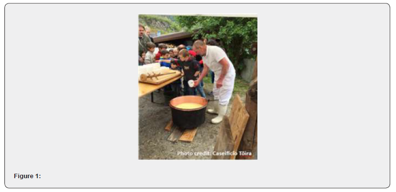
Switzerland has a long tradition linked to organic agriculture and sustainable food products, such as cheese, wine, and chocolate and, according to our research, these are the elements to be exploited to create a new value proposition involving sustainable tourism [10]. The cheese is one of Switzerland's signature products and having the possibility of making this culinary delicacy in a dairy can be a unique and funny experience for tourists [11]. For example, several dairies open their doors to tourists, allowing them to see how cheese is made and to actively participate in the production process. During the visit, tourists can also actively participate in the production of products, getting hands-on and helping the dairies prepare the cheese. This can be a very entertaining, engaging and educational experience, as visitors can see the cheesemaking process up close and have a first-hand experience of the art and tradition of cheese making [12]. Do we consider the satisfaction of eating a homemade cheese made by yourselves? (Figure 1)

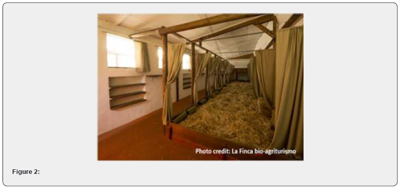
Another favourite practice of tourists traveling to Switzerland is sleeping on straw: this is a unique authentic experience in which tourists can try a form of traditional accommodation that may not be available elsewhere. This kind of ancestral experience allows visitors to immerse themselves in the local culture and learn about the traditions and practices of the area they are visiting. "Sleep in Straw" is a Swiss association which, among various activities, aims to promote this unique experience. On their website there are listed - at the date of publication of this article - 59 farms that offer overnight stays in straw beds (Figure 2).

The approach of various wine producers in the Mendrisio area - located in the southern part of Switzerland, in the canton of Ticino, near the border with Italy - is interesting, allowing tourists to have a unique experience, in close contact with nature, actively participating in the harvest. Several wineries welcome visitors and let them experience firsthand the magical festive atmosphere that traditionally accompanies harvest time by spending a day among the rows, picking bunches of ripe grapes, learning closely the first stages of winemaking. Enhancing the wine tourism experience leads to an enhancement in consumers' attitudes towards wine, their assessment of both extrinsic and intrinsic attributes, and their loyalty towards various wines. Moreover, segmenting consumers based on their level of wine tourism experience can assist wine marketers in comprehending their target audience and market direction [13].

Conclusion

Because of its history, its geography and its tradition, Switzerland has many opportunities to offer sustainable tourism thanks to its natural resources but, above all, thanks to a culture of sustainability that also passes through its agriculture and its sustainable food products. Switzerland can continue to be an ideal tourist destination for those seeking an authentic and sustainable experience but has to innovate new tourist proposition to be more captivating and contemporary like Regenerative Tourism (that aims to regenerate and restore the natural and cultural systems of local communities) or New Technologies (changing the tourism industry worldwide, including agriculture and rural tourism) with mobile apps and artificial intelligence that are leading to greater transparency, user engagement and personalized services for travellers.

By embracing this new approach, Switzerland can ensure the long-term viability of its tourism industry while preserving its pristine environment and unique cultural identity.

To Know More About International Journal of Environmental Sciences & Natural Resources Please click on:

For more Open Access Journals in Juniper Publishers please click on: 

Wednesday, May 15, 2024

ASPEN Study Case: Real Time in Situ Tomato Detection and Localization for Yield Estimation - Juniper Publishers

 Agricultural Research & Technology - Juniper Publishers


Abstract

As the human population continues to grow, our food production system is challenge. With tomato as the main fruit produced indoors, the selection of varieties adapted to specific conditions and higher yields is an imperative task if we are to meet the growing food demand. To assist growers and researchers in the task of phenotyping, we present a study case of the Agroscope phenotyping tool (ASPEN) in tomato. We show that when using the ASPEN pipeline, it is possible to obtain real-time in situ yield estimation without a previous calibration. To discuss our results, we analyse the two main steps of the pipeline in a desktop computer: object detection and tracking, and yield prediction. Thanks to the use of YOLOv5, we obtain a mean average precision for all categories of 0.85, which together with the best multiple object tracking (MOT) tested allow obtaining a correlation value of 0.97 compared to the real number of tomatoes harvested and a correlation of 0.91 when considering the yield thanks to the use of a SLAM algorithm. In addition, the ASPEN pipeline demonstrated to be able of predicting subsequent harvests. Our results demonstrate in situ and real-time size and quality estimation per fruit, which could be beneficial for multiple users. To increase the accessibility and use of new technologies, we make publicly available the necessary hardware material and software to reproduce this pipeline, which includes a dataset of more than 820 relabelled images for the tomato object detection task and the trained weights

Keywords: Tomato; Yield; Food production system; Phenotyping; Agricultural industry; Fruit detection

Abbreviations: MOT: Multiple Object Tracking; UGV: Unmanned Ground Vehicles; NN: Neutral Networks; LIDAR: Light Detection and Ranging; SFM: Structure from Motion; SLAM: Simultaneous Localisation and Mapping; ASPEN: Agroscope Phenotyping Tool; CNN: Convolutional Neural Network; GUI: Graphical User Interface; GFLOPS: Giga Floating-Point Operations Per Second; ROI: Region of Interest; RSE: Residual Standard Error

Introduction

As we approach the estimated inflection point of the world population growth curve UN, increasing global food availability is more important than ever. Especially with the current climate crisis threatening our food system Owino et al. [1]. Several strategies have been applied throughout the food production chain to address this issue FAO [2]. To this end, new methods have been tested across the agricultural industry to speed up results and increase efficiency, particularly in new technologies in a so-called fourth agricultural revolution, even though the impact of these new technologies is not clear Barret & Rose [3]. The vast majority of these new methods require large amounts of information obtained directly from the field or plants, in descriptive processes called phenotyping. Phenotyping is the activity of describing, recording or analysing the specific characteristics of a plant and due to the nature of this process and the required frequency, it is a time-consuming task Xiao et al. [4]. While the principle of phenotyping is not new, the quantity and quality of information that is today been generated has never been seen before, making imperative to reduce the time required for this task. Remote sensing has been used and its automation has already been demonstrated thanks to new algorithms and technologies Chawade et al. [5], even further opening up new opportunities for real-time data utilisation, what could save resources and further improve the industry as a whole Bronson & Knezevic [6].

There are several ways to automate phenotyping, with each path depending on the allocated budget and working conditions. For example, Araus et al. [7] divide these paths according to the distance to the target. Satellites can be used with fast data acquisition per m2, but with a trade-off between resolution and investment costs. Other methods closer to the plants, such as stationary platforms, allow for higher spatial resolution data, but are less flexible and more expensive to implement. A proven solution is the use of drones, which are more flexible than fixed platforms, but still not as flexible as they cannot work in covered crops. On the other hand, handheld sensors, manned or unmanned ground vehicles (UGVs) are more flexible than the aforementioned platforms and have a higher resolution, a lower initial investment, but can cover smaller areas than the previously mentioned methods. The effectiveness of this last category has been well demonstrated, especially in the fruit detection and localisation tasks e.g. Scalisi et al. [8], but affordable open-source alternatives are scare. The phenotyping subtask of fruit detection in images was initially based on shape and colour, until the advent of neutral networks (NN), which were particularly advanced after 2012 e.g. Hinton et al. [9]. These have led to more robust results in fruit detection.

Today, well-established algorithms such as RCNN Girshick et al. [10], Mask-RCNN He et al. [11] and YOLO Redmon et al. [10] are constantly used for research purposes and in production environments. For example, Mu et al. [12] show that when using RCNN, they could achieve a mean average precision at 0.5 intersection over union (IoU) (mAP@0.5) of 87.63%, which later correlates with the real number of tomatoes per image at 87%. Other authors, Afonso et al. [13]; Seo et al. [14]; Zu et al. [15] showed that when using Mask-RCNN, focused on the task of instance segmentation, they obtain a similar or higher average precision than Mu et al. [12], with values of mAP up to 98%, 88.6% and 92.84% respectively in each study. These previous works demonstrate the ability of the presented algorithms not only to detect objects, but especially to detect individual tomatoes in situ. A notable point of these works is that the comparability of their results is technically incorrect since each detection algorithm was trained on different image datasets. To compensate for this, a standardised dataset must be used and although some few datasets are freely available online to train machine learning algorithms in the task of tomato object detection, these are rarely used. Remarkable datasets are "laboro tomato" Laboroai [16] and "tomatOD" Tsironis et al. [17] due to its quality and availability.

Although the previously mentioned NN based algorithms have good detection rates, they are not capable of running in real time (more than 30 frames per second, FPS). For example, using a variant of R-CNN, Faster R-CNN, Seo et al. [14] achieve up to 5.5 FPS using a desktop computer equipped with a graphics processing unit (GPU) card (NVIDIA GTX 2080 ti), without mentioning the input size of the model. Thanks to the introduction of YOLO, Liu et al. [18] have shown that near real-time analysis is possible. In their case, the authors improved the YOLOv3 model by using a denser architecture and round boundary boxes that better fit the shape of tomatoes. These changes allowed them to achieve an F1 score, a weighted average of precision and recall, of 93.91% at a speed of 54 ms (18 FPS), compared to 91.24% at 45 ms (22 FPS) and 92.89% at 231 ms (4.3 FPS) for the original YOLOv3 and Faster R-CNN, respectively. In their case, images of 416x416 pixels were processed on a desktop computer equipped with a GPU (NVIDIA GTX 1070Ti). With a faster, more robust and more recent version of YOLO, YOLOv5, Egi et al. [19] achieve an F1 score of 0.74 for red tomatoes, which correlates at 85% with a manual count. Although no speed was documented in their work, the various algorithms of YOLOv5 are capable of running in real time at resolutions below 1280 pixels, depending on the system used (CPU vs. GPU) and model implementation Jocher et al. [20]. In addition, Egi et al. [19] demonstrate that the use of a state-of-the-art multiple object tracking (MOT) algorithm allows each individual object to be tracked along a video sequence.

For the tracking task, several MOT algorithms have been proposed, among which we highlight SORT Bewley et al. [21], bytetrack Zhang et al. [22] and OCSORT Cao et al. [23] as their code is publicly available, they have a high performance and they can run in real time in a common CPU unit even in the presence of multiple objects. Once an object has been detected, it needs to be located in space, which can be done in a number of ways. One simple way is to use RGBD cameras that contain a deep channel (D). This information can be used to distinguish the foreground from the background objects, which has been well demonstrated in tomatoes by Afonso et al. [13], allowing for object localization within frame, but missing the global position of the detected objects. Using an alternative methodology, Underwood et al. [24] show that it is possible to reconstruct a non-structural environment using Light Detection and Ranging (LiDAR) technology for within frame, together with GPS data for global localization in a post-processing method. Thanks to their method, they were able to locate and estimate almond yield at tree level with an R2 of 0.71.

The use of 3D reconstruction techniques has been less explored in greenhouses. Masuda et al. [25], show that tomato point clouds obtained from structure from motion (SfM) can be further analysed to obtain per plant parameters such as leaf area, vapour length using a 3D neutral network, Pointnet++ Qi et al. [26], with an R2 of 0.76 between the ground truth area and the corresponding number of points.

In a more advanced analysis, Rapado et al. (2022) show that by using a 3D multi-object tracking algorithm, that really in an RGB camera and LiDAR, they achieve a maximum error of 5.08% when localising and counting tomatoes at a speed of 10 FPS. Similarly, other authors have documented that by the year 2022, pipelines based on existing 3D neural networks are slower than 2D methods that really in additional sensors to obtain deep information (e.g. Afonso et al. [13], Ge et al. [27]. In addition, actual 3D neural networks have major limitations such as maximum input size, large number of parameters that make them slower to train, high memory consumption, and moreover, they are particularly limited by the lack of datasets for training reasons Qi et al. [28].Nevertheless, new low-cost 3D pipelines and datasets are constantly being released to increase the availability of this technology (e.g. Schunck et al. 2022, Wang et al. [29].

In order to correlate these detections with real yields, 3D localisation is required, and remarkably, simultaneous localisation and mapping (SLAM) algorithms have not been widely used in agricultural environments, possibly due to their lack of robustness Cadena et al. [30]. Previous SLAM methods are suitable for more structured environments, with clear corners and planes that allow incoming LiDAR scans to be aligned, which can be used for localisation (LiDAR odometry, LIO). A possible solution for unstructured environments is to use images for localisation (visual odometry, VIO), but this tends to fail in fast motion. Sensor fusion, a technique that fuses multiple sensors together, can provide more robust systems that can, for example, align incoming LiDAR scans when using VIO for navigation. This technology is better suited to environments that lack clear features, such as outdoor environments. Notable examples of these algorithms due its robustness and open source code include VINS-FUSION Qin et al. [31], CamVox Zhu et al. [32], R3Live Lin & Zhang [33], and FAST-LIVO Zheng et al. [34].

The low use of these technologies in the agricultural sector, either separately or together, could be attributed to several reasons, including the maturity of the technologies, budgetary reasons, and a knowledge gap between farmers and computer science e.g. Kasemi et al. [35]. The Agroscope Phenotyping Tool (ASPEN) aims to break the digital phenotyping barrier among agricultural researchers, thanks to a proven and affordable pipeline that can work in situ and in real time for fruit detection, allowing non-experts to use the tool. In this paper, we demonstrate that this pipeline: 1) allows 3D reconstruction of a non-structured environment using a SLAM algorithm, and thanks to this 2) can localise and describe tomato fruits in a traditional greenhouse thanks to the addition of an object detection algorithm. Most importantly, in order to increase the accessibility and use of this pipeline, we are making the necessary hardware and software to reproduce it publicly available, which we hope will help to bridge the gap between agricultural and computer scientists.

Materials and Methods

Hardware and Software

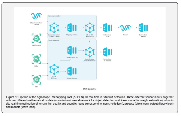
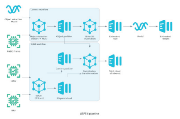
An ASPEN unit was used to evaluate the ASPEN pipeline (Figure 1). Although it is not the aim of this paper to discuss the configuration or selection of the equipment used, a brief description is given below. For more details, the reader is invited to refer to the online project repository (https://github.com/camilochiang/aspen, Chiang et al. in preparation). The ASPEN pipeline considers a set of input sensors connected to an embedded computer using the robot operating system (ROS, Stanford Artificial Intelligence Laboratory et al. 2018), version melodic in a gnome-based version of Ubuntu 18.04.6 LTS, with the aim of reconstructing and locating plants, fruits or diseases in situ in real time, where we here focus in the fruit case. ASPEN uses a specific selection of sensors and electronic components that may already be present in an agricultural research facility. To achieve this goal, the system relies on two main workflows, tightly coupled and orchestrated by an embedded computer equipped with a GPU (Jetson Xavier NX 16 Gb): the camera workflow and the SLAM workflow.

For the camera workflow, a synchronised RGBD without timestamp synchronisation (Realsense, R415 - 1920x1080 pixels at 30 FPS with synchronised depth) is processed with a convolutional neural network (CNN) object detection technique based on the RGB. Once that a model has been selected and object detection per frame has been performed, each object is identified and tracked using a multi-object tracking (MOT) algorithm were an unique ID is assigned. Finally, once the detected tracked object passes a region of interest (ROI) of the field of view and it is confirmed as a unique object who have not been register before, its localisation within the image is transferred to the 2D to 3D estimation node. Using the localisation given by the MOT algorithm for each object, the 2D to 3D estimation node uses the deep (D) frame information to estimate the dimensions (mm) of the tracked object and its localization with respect the camera position. For each object detection, the minimum distance to the camera is extracted and then the actual diameter is calculated and used by a dimensional model (Figure 1) to convert to weight (g).

In addition to this workflow, two other sensors, an Inertial Measurement Unit (IMU, BMI088 bosh) and a Light Detection and Ranging (LiDAR, Livox mid-70, configured into single return mode) unit, as well as the RGB channels of the RGBD camera, are used in the parallel SLAM workflow who allow to locate each RGBD frame within a global mapping and therefore each tracked object in a 3D map. These sensors were choose due its low cost compared with similar sensors, and in case of the LiDAR especially due the extreme low minimum detection range (5 cm). The aim of this workflow is to reconstruct the environment in which the tomatoes are located and to provide a relative position for each tomato (with respect to the initial scanning point), which will then allow the detected tomatoes to be correlated with the handmade measurements. For this task, R3Live Lin & Zhang [33] was chosen as the SLAM algorithm, as it attaches new incoming points from the LiDAR unit (10 Hz) using the IMU (200 Hz) and image information and does not really only use LiDAR features for this task and can run in real time (faster than 30 FPS). These characteristics, shared with other similar visual odometry algorithms (VIO), show in our preliminary research to work better in agricultural environments in collaboration with SLAM algorithms that rely only in LiDAR odometry (LIO) (data not shown), potentially due to the clear lack of features (corners, planes) in a so-called "unstructured environment", which makes LIO algorithms more difficult to converge. To allow reproducibility, the input from all sensors are recorded within the ASPEN unit. A simple graphical user interface (GUI) is available to facilitate this task.

Experiments

To evaluate the ASPEN pipeline in the specific task of tomato detection and localisation, we started by training YOLOv5. Five different models (n, s, m, l and x) from the YOLOv5 family were trained at two different resolutions: 512 (batch size 20) and 1024 (batch size 6) pixels up to 300 epochs. These models differ mainly in the complexity of the model architecture, with the simpler models aiming to operate under resource-constrained conditions, such as mobile phones and embedded computers. This network was trained using 646 images for training and 176 images for validation, coming from our own datasets and other open source datasets (laboro-tomato and tomatoD). Regardless of the origin of the dataset, tomatoes were re-labelled in three different categories: immature, turning and mature tomatoes, with approximately 3500, 1000 and 900 instances of each category, respectively. After training, one of the resolutions and one of the models were selected for a posteriori use. For details of the dataset, the reader is invited to visit the online repository.

Once the model that met our requirements and had the best performance had been selected, two commercial-type greenhouses in the facilities of Agroscope (Conthey, Switzerland), with tomatoes of the Foundation variety grafted on DRO141, were scanned with an ASPEN unit on three consecutive harvest days in the middle of the production period of 2022. Each scan lasted a maximum of 12 minutes and was performed close to midday to ensure similar light conditions. Each greenhouse of approximately 360 m2 contained eight rows of tomato plants, each row 25 m long. The six central rows were scanned sequentially, with both sides of each row scanned before moving on to the next row. These rows were also divided into 3 blocks for other experiments, with buffer plants at the beginning, between blocks and at the end of each row. The scans were recorded as bag files using ROS. The resulting bag files were then transferred to a desktop computer (Lenovo ThinkPad P15, Intel core i9, GPU NVIDIA Quadro RTX 5000 Max-Q, 16VGb) for reproductive and posterior analysis. The analysis was automated with the aim of detecting tomatoes per block. To do this, the videos were first reviewed and pre-registered with timestamps of the transition between blocks.

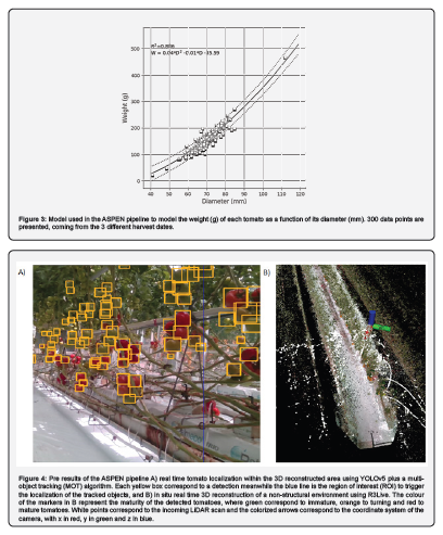
To validate our results, after each scan we harvest all the tomatoes ready for marketing. Harvesting was done per bunch, usually from 4 to 5 tomatoes, which occasionally led to the harvesting of turning tomatoes. Harvesting took place either on the same day or the following day after each scan. To increase the spatial resolution of the validation data, each row was harvested side-by-side and each row was further divided into three different blocks, resulting in 216 validation points. This was incorporated into the analysis using a distance filter with the D-frame of the RGBD camera, ignoring any objects detected more than 50 cm from the ASPEN unit, as these correspond to elements in the background or on the other side of the row. For each harvest, the total weight was measured, including the weight of the pedicel. Differently, the number of fruits was counted per block only, regardless of the side of the row, giving 108 validation points. To build the size-to-weight model shown in Figure 2, after each scan, 100 tomatoes were harvested from the non-scanned rows belonging to the three categories mentioned above. These tomatoes were measured and weighted, and the model used later for yield estimation is shown in Figure 3.

To complement the validation of the ASPEN pipeline, three MOT algorithms were tested under similar implementation frameworks and parameters (Python 3.8): SORT Bewley et al. [21], Bytrack Zhang et al. [22], and OCSORT Cao et al. [23].The quality of the yield estimation results depends not only on good object detection, but also on correct tracking along the frames until each object reaches a region of interest (ROI), where it is counted. Independently of the MOT algorithm used, an estimated position, size and weight was calculated for each tomato detected. An example of the detection and reconstruction process is shown in Figure 4. The correlation of the three different MOT algorithms with weight and count in relation to the real harvest is shown in Figure 5.

Statistics

A priori and posteriori statistical analyses were performed using Python 3.8 Van Rossum & Drake [36] and the Statsmodels package (version 0.13.5, Seabold & Perktold [37]. A quadratic equation was fitted to the size-weight relationship (Figure 3), as this statistically fit the data better than a simpler relationship (data not shown). To estimate the correlation between crop yields, either in number or weight, a linear correlation without intercept was fitted between the manually measured data and the estimated data from the ASPEN pipeline, considering each crop subsample as a data point (n = 108 for the number task and n = 216 for the weight task). To evaluate the ability of the ASPEN pipeline to predict future yields based on previous measurements, we correlate the estimated number of tomatoes in the turning category with the following 3 harvests for each subsample as a data point (n = 108). Finally, to evaluate the task of size measurement, an f test of the size distribution was carried out within each category (Figure 6).

Results

Object detection

Within the ASPEN pipeline, the first task in the camera workflow is object detection (Figure 1), which requires a previously trained object detection model. As shown in Figure 2, when evaluating the task on the desktop computer using the family of models of the YOLOv5 algorithm (n, s, m, l and x models with 4, 16, 48, 109 and 207 Giga floating-point operations per second, GFLOPS), at a resolution of 512 pixels (px), an increase in the complexity of the model used allows a higher mean average precision at interception over union of 0.5 (mAP@0.5), which is particularly the case between the first two models (nano;n vs. small;s). Subsequently, more complex models (medium; m, large; l and extra-large; x) did not contribute to a higher mAP@0.5. In contrast to the lower resolution results, a higher resolution of 1024 px results in higher mAP@0.5 values for simpler models. At 512 px, the improvement in mAP values due to higher complexity was close to 2% between the two simpler models (n vs s), while a higher resolution contributed up to 5% improvement in mAP@0.5 values between the two n models.

Selecting the simplest model, YOLOv5n, also reduced the inference time from 8 ms to 25 ms compared to the more complicated model (x). Figure 2B shows the precision-recall curve of the selected model (YOLOv5s at 1024 px). The F1 values, a weighted average of precision and recall ranging from 0 to 1, were 0.941, 0.777 and 0.838 for the immature, turning and mature categories at mAP@0.5, with an average F1 value of 0.852 across categories. Irrespective of the category, the main difficulty was with precision measurement, suggesting a high number of false positives. Although the mature category had a similar number of cases to the turning category (around 900 compared to 1000), it is interesting to note that the turning category is still the most difficult to discriminate. On the other hand, the green category has a higher F1 value with more than 3500 instances.

Size to weight model and localisation

The next step was to investigate weight estimation using manual diameter measurements. For this purpose, a linear model represented by a parabolic function was used, as this one fitted our data better than other functions (data not shown). This correlation, with an R2 of 0.886, holds regardless of the ripeness of the tomatoes (data not shown) and when considering the production of layers of either small or large size, as shown in Figure 3. The average weight of the tomato samples was 147 ± 2 g (standard error, SE), which corresponded to the average weight of the harvested tomatoes during the scanning process.

Localisation estimation

To illustrate the localisation process, an example scan is shown in Figure 4. Figure 4A shows the object detection where different tomatoes are marked in boxes. These objects were then tracked using one of three different multi-object tracking (MOT) algorithms and once they passed a region of interest (blue line in Figure 4, they were registered, localised and measured in 3D space as shown in Figure 4B using the D channel from the RGBD camera, the size-to-weight model (Figure 3) and 3RLive. The selection of the region of interest (ROI) boundary was based on previous work in fruit detection (e.g. Borja and Ahamed, 2021) and an observed better object detection even in the presence of occlusions, as the objects were closer to the camera.

ASPEN pipeline validation

The number of tomatoes detected and their respective calculated weight is shown in Figure 5, in relation to the number of tomatoes harvested and their weight. It can be seen that both MOT algorithms of the SORT family underestimated the number and/or the total weight of tomatoes, while the bytetrack algorithm strongly overestimated both parameters. In addition, the bytetrack algorithm produced a significantly higher residual standard error (RSE) for both measurements compared to the SORT family algorithms. No statistical difference was found between the SORT algorithms independent of the measured variable. Independently of this, OCSORT was chosen as the best MOT algorithm due to a lower RSE. The size distribution of a manual measurement compared to the automated procedure is shown in Figure 6 for the OCSORT MOT algorithm. The distribution of measurements from the automated method did not differ from the manual method, regardless of the tomato category. On average, the ASPEN measurements were slightly lower than the manual measurements, but similar dynamics could be observed, with green tomatoes having higher mean diameter values (60 vs 56 mm) and a wider distribution, turning tomatoes having a lower mean value (62 vs 67 mm) and a skewer distribution, and ripe tomatoes also having lower mean values (64 vs 69 mm) and a similar distribution compared to the manual measurements. When correlating the number of turning tomatoes with the actual harvest and the next three harvests, the highest correlation was found when using OCSORT. Regardless of the MOT algorithm used, these correlations were weaker over time and have an increasing RSE. The third harvest was an exception, where a slight increase in the average correlation was observed (Table 1).

Discussion

The results presented here validate the use of ASPEN for tomato yield estimation. Although several previous studies have demonstrated the capability of image analysis using machine learning approaches, it was not until the introduction of YOLOv5 Jocher et al. [38] that real-time image analysis was possible. Mu et al. [12] showed that using R-CNN could achieve a mAP@0.5 of 87.83% when training on a category of tomatoes, and the detections correlated at 87% when compared to manual counting on the same images. Seo et al. [14] found 88.6% of tomatoes in images using a faster version of R-CNN: Faster R-CNN. In their case, they were also able to classify into six different categories, which took a total of 180 ms (5.5 FPS) per image on a computer equipped with a GPU. After the introduction of YOLOv3, near real-time results have already been achieved. Liu et al. [18] show that modifying YOLOv3 for the tomato object detection task allowed them to increase the F1 score from 0.91 to 0.93 with a small increase in inference time from 30 (33 FPS) to 54 ms (18 FPS) for images of 416 x 416 pixels. In their case, these changes were due to a denser mesh and a circular bounding box that allowed higher mAP@0.5. Using RC-YOLOv4, a more recent and modified version of YOLO, Zheng et al. [34] achieve an F1 score of 0.89 with a speed of 10.71 FPS on images of 416 x 416 pixels in a GPU equipped computer, suggesting that the improvement between YOLOv3 and YOLOv4 is mainly due to the gain in detection quality and not to the speed of the algorithm.

More recently, and similar to our work, Egi et al. [19] demonstrated that a flying drone with side view, using the latest YOLOv5 together with DeepSORT as MOT tracker, could achieve an accuracy of 97% in the fruit counting task in an average of two tomato categories, and a 50% accuracy in the flower counting task. Notably, their paper does not mention the speed of the various steps involved. These previous works demonstrate the capacities of previous and current algorithms for tomato fruit detection, where our work aligns with these results at similar F1 scores and shows how these capacities have increased over time and can be applied to the task of tomato fruit detection. Although not perfect, see Figure 4 for a clear tomato occlusion, we were able to correlate the number of tomatoes with the actual harvest to 97% in real time using YOLOv5 without prior calibration of the method, and thanks to the speed of the algorithm we were able to further improve the results. A limitation of YOLOv5 is the lack of subcategories, which could improve the detection efficiency. Training the same dataset with the same model and resolution (YOLOv5s), but with only one category, achieved a higher F1 score of 0.95 (data not shown) compared to three categories (F1 value of 0.852).

This suggests that our pipeline could be further improved by adding a second step classifier after the object detection algorithm, without losing real-time capacity. To further improve not only the count but also the weight correlation, it is also possible to use instance segmentation algorithms e.g. Zu et al. [15], Fawzia & Mineno [39], Minagawa & Kim [40]. This change may increase the accuracy of the weight model, as only the area of each tomato is detected, which should remove many errors in size measurement, especially those due to occlusion or overlap. So far, the speed of this task has been the limiting factor for real-time instance segmentation, but newer and faster algorithms may allow better results in our pipeline Jocher [20]. A negative effect of introducing an instance segmentation algorithm would be to increase the mathematical complexity of the size determination task, as it may be possible to fit a sphere into the D-frame Gené-Mola [41].

Several methods have been tested to determine the size and position of each fruit. Mu et al. [12] showed, similarly to our work, that it is possible to obtain dimensional features in tomatoes using an RGB camera, but due to the lack of a third dimension, their data was only displayed as pixels. Thanks to the addition of a deep (D) channel, Afonso et al. [13] were able to filter foreground objects from their Mask RCNN detections, while our work shows that we can not only filter foreground objects, but also obtain object characteristics in real time (Figures 4-6), which can be useful to study the growth dynamics of tomato fruits. In terms of speed, the use of the D channel to obtain sizes has been demonstrated to be the fastest method available in 2022. For example, Ge et al. [42] using the 2D boundary box output of an object detection algorithm together with the corresponding depth frame took between 0.2 and 8.4 ms compared to 151.9 to 325.2 ms when using a 3D clustering method. Similarly, Rapado et al. (2022) were able to reconstruct tomato plants using an RGB camera and LiDAR with multi-view perception and 3D multi-object tracking, achieving a counting error of less than 5.6% at a maximum speed of 10 Hz.

While other high quality methods have been tested in tomato plant reconstruction e.g. Masuda [25], these can be up to 100 times more expensive than lower cost and resolution methods Wang et al. [29] and cannot run in real time. Several studies have been carried out using SfM to evaluate lower cost 3D reconstructions in greenhouses, but thanks to the recent introduction of cheaper solid-state LiDAR technology, our pipeline is able to run in real time at a similar economic cost to SfM. The benefits of 3D reconstruction have been well demonstrated in tomato, e.g. Masuda [25] were able to correlate the actual leaf area and stem length of tomato plants with their respective number of points, which can be useful in the task of phenotyping. When using LiDAR technology, the chosen SLAM technique plays a crucial role. In our case, R3Live successfully reconstructed the unstructured environment on a desktop computer in real time (average of 24 ms for visual and LiDAR odometry), but it is important to mention that the algorithm has more than 25 parameters to be tuned and that under stress conditions (fast movements, camera occlusions and turning points) this one constantly fails to converge, weakening the whole pipeline. The main reason for the failure was identified as the lack of clear features, planes and corners, which are usually absent in unstructured environments, and further research is required e.g. Cao et al. [43]; Zheng et al. [34], especially when porting the pipeline to the embedded computer.

The robustness of the MOT algorithm and the selection of a good ROI are crucial for the object localisation task. In our case, with the same settings, both SORT algorithms perform better than Bytetrack, mainly due to a multiple ID assignment, demonstrating the importance of a good MOT algorithm selection for the yield estimation task. Although newer tracking algorithms have been tested in the tomato counting task e.g. Egi et al. [19], they can be slower than the simpler algorithms presented here, especially when tracking multiple objects. Regarding a good choice of ROI, Borja & Ahamed [44] show in pears that a ROI located in the central part of the image gives the best results in their case. In our case, we observe that a ROI located at 75% of the image field of view gives the best results, since objects are closer to the camera, allowing the detection algorithm to make better predictions and reduce the probability of occlusions. Regarding the SORT algorithms, both were able to predict the amount or weight of the crop per experimental unit (Figure 5), but in an underestimated way. This could be partly explained by technical reasons or more practical ones. On the technical side, the lack of detection due to occlusion (Figure 4) or fruit leaving the field of view before entering the ROI could contribute to the error.

Meanwhile, practical reasons include the fact that tomatoes were harvested by bunch, which includes the occasional turning of tomatoes and the weight of the pedicel (with an average value of 50 gr per bunch). Independently, the addition of the D channel proved to be useful in capturing the size differences between categories (Figure 6) and reduced the uncertainty of the weight model by about 1 kg for the SORT models when compared to the product of the uncertainty of the count model and the average tomato weight. Although no difference was found between the size distributions, the slight difference between the sizes of the categories shown in Figure 6 may have contributed to the uncertainty of the weight model, but further investigation is required as the sample sizes were extremely different (300 manually measured vs. 27000 digitally measured tomatoes). Finally, our pipeline demonstrates the ability to additionally localise and predict future harvest based on the turning category, which, similar to our previous correlation results, has a higher correlation when using the SORT family of algorithms. Further research is needed to validate these claims.

To our knowledge, the results presented are the first example of real-time detection, characterisation and localisation of tomato fruit in situ and without calibration. Several experiments have been shown to work in post-processing with other fruits e.g., Underwood et al. [24], and as a result, commercial platforms are already available e.g., Scalisi et al. [8], Ge et al. [42]. These platforms can perform similar work, but they generally require a site/crop pre-calibration and do not have the flexibility presented here. The advantage of pre-calibration is that images can be captured at a faster rate, linked to GPS coordinates and therefore faster scanning speeds could be achieved, resulting in a lower price per m3 scanned. Although this is an excellent approach for commercial orchards where GPS connectivity is available and decisions can be made a posteriori, real-time data acquisition and processing allows decisions to be made in real time and in the field. The open source pipeline presented adds the flexibility of a terrestrial laser scanner that can work not only outdoors but also indoors. In addition, the lateral view of the crop and the higher image resolution may allow early disease detection when the ASPEN pipeline is coupled with a multispectral camera [45].

Conclusion

The present study demonstrates the capabilities of the ASPEN pipeline in the detection, characterisation and localisation of tomato fruits. Thanks to a series of sensors, we were able to reconstruct the scanned environment in real time, opening the doors to new developments and possibilities not only for the task of fruit detection, but also for other real time visual related measurements (e.g. disease and pest detection). In this study, the ASPEN pipeline correlated with the actual number and weight of harvested tomatoes at 0.97 and 0.91, respectively, and although the pipeline is not perfect, possibilities for improvement were discussed, especially with the aim of reducing the uncertainty of the method. Thanks to the 3D reconstruction of the environment, other physiological measurements could also be automated (e.g. leaf area, plant volume), but further research is needed, especially to compare these results of an affordable 3D scanner with high quality scanners. We hope that the presented results will stimulate agricultural researchers to work with new technologies, and to inspire this, we make publicly available the hardware material and software necessary to reproduce this pipeline, which includes a dataset of more than 850 relabelled images and models for the task of tomato detection.


To Know more about Agricultural Research & Technology: Open Access Journal

To Know more about our Juniper Publishers
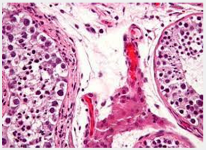
On the Positive Effects of Overconfident Self-Perception in Teams - Juniper Publishers

  Social Sciences & Management Studies - Juniper Publishers Abstract In this paper, we study the individual payoff effects of over confi...