Sero Prevalence of Bovine Foot and Mouth Diseases in Bale Zone Selected Districts Sinana and Agarfa Oromia, Ethiopia - Juniper Publishers

 Dairy & Veterinary Sciences - Juniper Publishers

Abstract

Ethiopia is country with the most abundant livestock population in Africa with an estimated domestic animal number of 56.71 million cattle. The Foot and mouth disease (FMD) virus is a highly contagious and economically devastating transboundary disease of cloven hooved domestic and wild animals. The Foot and mouth disease virus, the causative agent of foot and mouth disease belongs to the genus Pithovirus and the family Picornaviridae. It has seven sero types, namely: O, A, C, South African Territories (SAT) SAT1, SAT 2, SAT 3, and Asia.

The study was conducted from January 2022 to February 2022 in two selected districts of Bale zone namely Sinana and Agarfa which are in the administrative zone of Oromia Region, Ethiopia. The study populations were local and cross breed of cattle above the age of six months having no clinical symptom of any disease were included. A cross sectional study design was taking place to determine the sero-prevalence of FMD. The present study considered 50% expected prevalence, 95% confidence level and 5% absolute precision or marginal error. Whole blood samples each amounting to 8-10ml were collected from jugular vein of cattle using disposable needles and 10 ml non-heparinized vacutainer tube and 21 Gauge needle. The collected sera were tested by commercially available FMD NSP competitive ELISA kit (Non-structural proteins used as DIVA test) (ID Screen(r) FMD NSP Competition, ID-VET, Grabels, France) for the detection of antibody to 3ABC polyprotein. A total of 461 serum samples were collected and tested for FMD. Over all 103 samples gave positive results yielding a prevalence of 22.34%. Of the samples collected from Agarfa 25.97 % (60/231) were positive whereas of the 18.70% (43/230) samples collected from Sinana were found positive. The presence of this disease in the country is a major obstacle to the development of livestock resources because of its adverse effects on production and their product exports. An extensive regular surveillance and serotyping of FMD isolates throughout the country should be conducted to check the introduction and circulation of new serotypes in the country.

Keywords:Foot and mouth disease (FMD); sero-prevalence; competitive ELISA kit.

Abbreviations:FMD: Foot and Mouth Disease; SAT: South African Territories; FMDV: Foot and mouth disease virus; NSP: Non-Structural Proteins

Introduction

Ethiopia is country with the most abundant livestock population in Africa with an estimated domestic animal number of 56.71 million cattle [1]. The Foot and mouth disease (FMD) virus is a highly contagious and economically devastating transboundary disease of cloven hooved domestic and wild animals [2]. FMD is also among the most important livestock diseases that affects production and trade of animal and animal products in Ethiopia [3]. Sero-surveys done in different parts of Ethiopia reported FMD with different degrees of prevalence reaching up to 26% (6-9). Outbreak incidence studies have also indicated that FMD occurs throughout the country with significant variation in geography and production systems [3]. Among the seven serotypes of FMDV, four of them (O, A, SAT 2, and SAT 1) have been reported in Ethiopia in recent times [1].

The Foot and mouth disease virus (FMDV), the causative agent of foot and mouth disease (FMD), belongs to the genus Aphthovirus and the family Picornaviridae. It has seven serotypes, namely: O, A, C, South African Territories (SAT) SAT1, SAT 2, SAT 3, and Asia [4]. The highly infectious nature of the virus, the generation of high titers in respiratory secretions, the prolonged survival of the virus in secretions, the fast replication cycle, and the brief incubation time contribute to the virus’s rapid dissemination to fully susceptible populations. In addition to the animal-to-animal transmissions, FMDV is easily transmitted mechanically via fomites such as clothes, shoes, vehicles, and veterinary instruments [5]. Moreover, its spread is aggravated by uncontrolled movements of infected animals across geographic boundaries [6]. In Ethiopia, the disease has been affecting mainly cattle, while also causing problems in small ruminants at infrequent intervals [7].

Historically, the disease was first identified in 1957, but it had certainly been present in the country before that, since most livestock keepers were familiar with it and some were using traditional methods of immunization against it, such as “mouthing [7]. According to the report of [8] FMD serotypes O, A, and C were responsible for FMD outbreaks from 1957 to 1979. A separate report on the genetic characterization of FMDV from 1981 to 2007 disclosed additional serotypes such as SAT1 and SAT2. The occurrence of the disease leads to loss of production, restriction of exports, and other socio-economic problems in the area [9].

Direct impact of FMD includes meat and milk production losses, loss of drought power, lower weight gains, fertility problems, changes in herd structure, delay sale of cattle and products, and death of cattle, while the indirect impacts include additional cost of treatment, vaccination, vaccine delivery, movement control, diagnostic tests, culled cattle, and denied access to both local and international markets [10]. FMD currently is widely prevalent and distributed in all areas of Ethiopia across the different farming systems and agro ecological zones of the country. Previously, the disease used to frequently occur in the pastoral herds of the marginal low-land areas of the country. However, this trend has changed, and the disease is frequently noted in the central/ highland parts of the country [11]. Sero-prevalence investigations undertaken so far in the different parts of the country reported the prevalence that ranges from 5.6% to 53.6% in cattle [12]. In the current study area, knowing the status of the disease is very important because of a high cattle population and cattle marketing activities, the practice of communal grazing and watering and cattle movement.

FMD is endemic to most countries in sub-Saharan Africa and will not be eradicated from southern East Africa while infected buffalo are present except for few countries Southern Africa, where the disease is controlled by the separation infected wildlife from susceptible livestock as well as by vaccination. Largely due to the endemicity of the disease and the fact that FMD does not cause high mortality rates in adults’ animals which is (2%) and 20% in young animals. Several countries now realize that FMD is one of the transboundary diseases that should be controlled to ensure economic stability and access to lucrative international export markets for animals and animal products. Furthermore, they recognize that a regional approach would be needed to succeed [13]. Lack of movement control within countries and across international borders for both wildlife and domestic animals aggravates the problem and gives credence to the fact that FMD will remain a problem on the sub-continent for the foreseeable future [14]. Countries free of FMD impose strict import regulation on animals and animal products and potential viral contaminated fomites from FMD free countries. Greater loss can result from refusal from FMD free countries to import livestock and livestock products from endemic regions [15].

Several studies have been conducted on the sero-prevalence and associated risk factors of FMD in cattle in different parts of the country and still there is a scarcity of information in the study area. Implementing both sero-prevalence and associated risk factors investigation is crucial to generate baseline information about the disease in the selected Zone.
 Therefore, the objective of the present survey was to estimate the sero-prevalence and to assess associated risk factors of FMD sero-prevalence in Sinana and Agarfa districts.

Materials and Methods

Description of the Study Areas

The study was conducted from January 2022 to February 2022 in two selected districts of Bale zone namely Sinana and Agarfa which are in the administrative zone of Oromia Region, Ethiopia. Sinana is in Oromiya Regional State, Bale Administrative Zone. It is about 460 Km southeast of Addis Ababa and it has an altitude of 2400 m above sea level. It’s geographical from 07° 06’29’’ northern latitude and from 40° 12’52’’ eastern longitude. It has a bimodal rainfall pattern with the first peak from April to May and the second from August to October. The mean annual maximum temperature is 21.06°C and monthly values range between 19.39°C in October and 22.94°C in February. The mean annual minimum temperature is 9.32°C and monthly values range between 7.12°C in December and 10.81°C in April. The coldest month is December whereas February is the hottest month.

Agarfa district is found in the Bale Administrative Zone of Oromia Regional State, in Southeastern part of Ethiopia. It lays between 7°8’N to 7°28’N latitude and 39°31’E to 40°5’E longitude. The elevation of Agarfa district ranges from 1400 m to 3800 m above mean sea level (a.m.s.l). About 61% of the district is plain with slopes ranging from 0 to 8 degrees and most of this area lies in the southeastern and western parts of the study area. Wabe Shabelle river gorges and related rugged terrains make up about 31% of the district. Agarfa district falls within three traditional agro-climatic zones, vernacularly termed as Gamoji (hot), Badadare (temperate), and Bada (cold). Mean maximum and mean minimum temperatures are 25°C and 10°C respectively. The amount of maximum and minimum rainfall received in the area ranges between 1200 mm and 400 mm, respectively.

Study Populations

The study populations were local and cross breed of cattle above the age of six months having no clinical symptom of any disease were included. In addition, herd sizes considered were small, medium, and large as some of research handle the same way.

Study Design

A cross sectional study design was taking place to determine the sero-prevalence of FMD and associated risk factors in two selected districts of Oromia region and different herd sizes were included in the study based on the inclusion criteria. Semistructured questionnaires were administered to herd owners for the assessments of animal and herd level risk factors.

Sampling technique and Sample Size determination

Study districts were purposively selected based on higher study population, access to transportation and history of outbreaks for sero-prevalence determination and assessment of potential risk factors of FMDV. Individual animals from each herd were selected randomly as sampling unit to draw the required sample size. Since there was no previous study conducted on FMD in cattle found in the selected areas, the present study was considered 50% expected prevalence, 95% confidence level and 5% absolute precision or marginal error. Based on these assumptions, the total number of animals to be included in the study was determined using Thru field (2007) formula form the two Districts selected. The sample size was determined using the formula given as follows:
Where, N = required sample size, Pexp = expected prevalence, d² = desired absolute precision.

Sample Collection and Transportation

A total of 768 whole blood samples each approximately amounting to 8-10ml were collected from jugular vein of cattle using disposable needles and 10 ml non-heparinized vacutainer tube and 21 Gauge needle. Following whole blood sample collection, vacutainer tubes were labeled and transported to around veterinary clinic and kept overnight at room temperature to allow the blood clot at slant position. Correspondingly, each sample was identified along with sex, age, and district. Then, serum samples are transferred from vacutainer tubes to cryogenic vials and stored in -20°C refrigerator at Asela veterinary regional laboratory. The samples were tested using the FMD non-structural protein ELISA to determine if animals in the herd had been recently infected with FMD virus thereby estimating the sero-prevalence in the two selected districts.

Open and closed ended questionnaires were administered to herd owners to assess potential risk factors of the disease alongside sample collection. Respondents from each district were randomly selected and interviewed to assess potential risk factors of the disease. Study populations’ sex, age, herd size and district are considered as hypothesized risk factors for the occurrence of FMDV. Herd owners having cattle are the sampling units for questionnaire survey. All necessary epidemiological information was collected, tabulated, coded, and analyzed using suitable statistical analysis on individual animal bases.

Serological Diagnostic Test

The collected sera were tested by commercially available FMD NSP competitive ELISA kit (Non-structural proteins used as DIVA test) (ID Screen(r) FMD NSP Competition, ID-VET, Grabels, France) for the detection of antibody to 3ABC polyprotein which is a useful indicator of past FMDV infection regardless of the serotype involved. The 3-ABC-ELISA was used according to the manufacturer’s instructions. The test principle is the blocking of plate bound NSP antigen by antibodies present in the serum samples. Any antibody specific for 3ABC binds to the antigen in the wells and forms an antigen/antibody complex on the plate well surface. The antibody to the assay was performed according to manufacturer’s instruction and results were analyzed and interpreted.

Data Management and Analysis

Data generated from laboratory analysis and questionnaire survey were recorded and coded using Microsoft Excel spreadsheet (Microsoft Corporation) and analyzed using STATA version 13.0 and R studio. Descriptive statistics (frequency and percentage) were employed to calculate the proportion of risk factors for FMD. Individual level animal prevalence was calculated by dividing the number of animals with positive ELISA tests by the total number of tested animals. In all the analyses, confidence levels at 95% were calculated, and a P < 0.05 was used for statistics.

Results

Prevalence of FMD in the samples

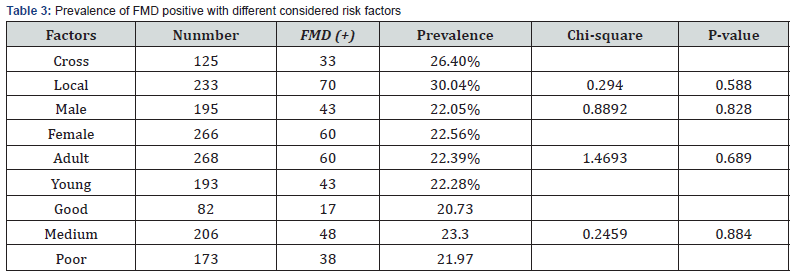
total of 461 serum samples were collected and tested for FMD. Over all 103 samples gave positive results yielding a prevalence of 22.34 %. Of the samples collected from Agarfa 25.97 % (60/231) were positive whereas of the 18.70% (43/230) samples collected from Sinana were found positive as described in table 1 below. At the kebele/Peasant Association level 18.25%, 19.23%, 26.78% and 25.21%of the samples collected from Alemgena, Kasoshek maro, Makora chafe, kasomaro, respectively gave positive results for FMD as shown in table 2 below. From tested samples for FMD cross breeds were 26.40% and local breeds were 30.04% as shown in table 3 below. Risk factors such as breed, sex, age, and body conditions were considered. Higher sero-prevalence was recorded in local breed cattle with prevalence of 30.04 %. Cattle with medium body condition have higher sero-prevalence 23.3%. Sex and age show almost nearly the same result.

Discussion

The overall sero-prevalence rate of 22.34% reported in this study agreed with the previous finding from Ethiopia [16] in which sero-positivity of 26.5% was reported. Compared to the present findings lower prevalences of 5.6% [17], 8.01% [18] and 9% [19] were reported from Afar Regional State, Dire Dawa and western Ethiopia, respectively. On the other hand, relatively higher seroprevalence was previously reported in samples from the Eastern zone of Tigray with 41.5%; followed by the Guji zone of Oromia and Yeka district of Addis Ababa city, with 32.7% and 30% respectively [20]. [21] in Sudan, [22], in Saudi Arabia and Uganda also reported sero-prevalences of 16%, 53% and 77% respectively, from FMD virus infected cattle. The observed prevalence variation may be resulted from differences in individual animals breed, age, and sex and production system.

To Know more about Journal of Dairy & Veterinary Sciences

Click here: https://juniperpublishers.com/jdvs/index.php

To Know more about our Juniper Publishers

Click here: https://juniperpublishers.com/index.php

Tapping the Potential of Modulated Light to Ward off Pathogens - Juniper Publishers

 Biotechnology & Microbiology - Juniper Publishers

Abstract

Antimicrobial resistance of pathogens poses a significant challenge to public health worldwide which necessitates urgent innovative approaches for infection control. The interplay between light and biological organisms has been a subject of interest for decades. In recent years, modulated light has gained attention as a potential tool for combating pathogens. This short paper appraises the possibility of using modulated light, specifically light with a controlled variation in intensity or wavelength, as a weapon against harmful microorganisms.

Keywords: Modulated Light; Pathogen; Inactivation; Wavelength; Microorganisms

Introduction

The battle against infectious diseases is a constant one, with the emergence of antibiotic-resistant bacteria highlighting the need for novel approaches. In recent years, research has explored the potential of light-based disinfection to inactivate pathogens. Recent advancements suggest that modulated light can influence pathogen behavior and host resistance, potentially serving as a non-invasive method to combat infections. The rise of antimicrobial resistance has underscored the need for novel strategies to combat infectious diseases. Traditional antimicrobial agents, while effective, often encounter challenges such as resistance development and toxicity. As such, researchers have turned to alternative approaches, including phototherapy, as a promising avenue for infection control [1-4]. Modulated light, characterized by its specific frequency and intensity, has emerged as a particularly intriguing option due to its ability to target pathogens while minimizing harm to host tissues. In this paper, we delve into the potential of modulated light as a non-invasive, cost-effective, and environmentally friendly tool for warding off pathogens. Light has long been known to affect the biological rhythms and physiological processes of living organisms. The concept of using light modulation as a defense against pathogens is gaining traction, with evidence suggesting that certain wavelengths and intensities can inhibit pathogen growth and virulence [5-10]. This paper explores the mechanisms by which modulated light affects pathogens and discusses its implications for future therapeutic strategies. This paper explores the promising role of modulated light in disrupting microbial growth and survival, highlighting its mechanisms of action and potential applications in diverse settings. Through a review of recent studies, the effects of modulated light on various microorganisms are elucidated and we discuss its advantages, limitations, and future directions in the field of infection control.

Mechanisms of Action

Photodynamic Inactivation

Photodynamic inactivation involves the use of light-sensitive compounds that, when activated by light, produce reactive oxygen species (ROS) that can damage cellular components of pathogens, leading to their inactivation. Light of a specific wavelength activates photosensitizing agents inducing oxidative damage to microbial cells. This oxidative stress disrupts essential cellular components, leading to cell death. Alternatively, in photothermal therapy (PTT), modulated light is absorbed by photosensitive materials, causing localized heating and thermal ablation of microbial cells. Additionally, modulated light can interfere with microbial biofilm formation and quorum sensing, further impeding pathogenicity. Visible light (400-700 nm) is generally considered non-hazardous. Studies have shown that pulsed visible light, particularly in the blue spectrum (400-470 nm), can inactivate bacteria, viruses, and fungi. The exact mechanism of action remains under investigation [5-10].

Circadian Rhythms and Immune Response

Circadian rhythms regulate various physiological processes, including the immune response. Modulated light can synchronize these rhythms, potentially enhancing the host’s immune response to pathogens [7].

Chromophore Targeting

Certain studies suggest that modulated light, specifically visible light with specific pulsing patterns or narrow wavelengths, may offer a safer and potentially more targeted approach. As for instance, certain pathogens possess chromophores, molecules that absorb specific wavelengths of light. By targeting these chromophores with modulated light at their absorption peaks, it might be possible to selectively damage the pathogen without harming surrounding healthy cells [8-9].

Merits

This therapy possesses certain merits which are listed below.

· Safety: Compared to UV-C, visible light poses less risk to human health.

· Specificity: Targeting chromophores could allow for selective inactivation of pathogens.

· Non-invasive: Light-based disinfection can be applied remotely, minimizing the need for direct contact with contaminated surfaces.

Challenges and Future Directions

Despite its promise, modulated light therapy faces several challenges that warrant further research. Optimization of treatment parameters, including light dosage and delivery methods, is essential to maximize efficacy and minimize adverse effects. Moreover, elucidating the underlying mechanisms of action and potential resistance mechanisms is crucial for the development of targeted therapies. Additionally, studies evaluating the safety and long-term effects of modulated light therapy in clinical settings are needed to establish its feasibility and efficacy for widespread use. Future research efforts should focus on expanding our understanding of modulated light's antimicrobial properties and exploring its applications in diverse settings, including healthcare facilities, food processing, and water treatment.

However, significant challenges remain:

· Optimizing Parameters: The effectiveness of modulated light likely depends on various factors, including pulse frequency, wavelength, and total light dose. Research is needed to identify the optimal parameters for different pathogens.

· Efficacy in Real-World Settings: Laboratory studies have shown promising results, but translating this to real-world scenarios with diverse microbial communities requires further investigation.

· Cost and Implementation: Developing and deploying light-based disinfection systems necessitates cost-effective light sources and practical implementation strategies.

Although light modulation underscores its potential as deterrent for microbes, there is still a long way to go. Understanding the precise mechanisms by which modulated light can lead to effective inactivation of microorganisms is mandatory. Only, a better grasp of interplay of modulated light with microbe can make this area more prominent. Along side of it, the incorporation of combination therapies such as disinfection methods, like chemical disinfectants with modulated light results in synergistic effects. Another formidable challenge is the design as well as fabrication of cost-effective and power efficient light which can cater to specific and selective disinfection is extremely important leading to wider adoption.

Conclusion

Modulated light holds promise as a novel and potentially safer approach to pathogen control. While significant research is needed to address existing challenges, this technology presents exciting possibilities for the fight against infectious diseases. Its non-invasive nature and potential to reduce reliance on antibiotics make it an attractive option for further research and development. By leveraging its unique properties, including specificity, versatility, and non-invasiveness, modulated light has the potential to revolutionize infection control strategies. Continued research efforts are needed to optimize treatment protocols, validate efficacy in clinical settings, and address remaining challenges. With further advancements, modulated light therapy could emerge as a valuable tool in the fight against antimicrobial resistance and infectious diseases.

To Know More About Advances in Biotechnology & Microbiology Please click on:

https://juniperpublishers.com/aibm/index.php

For more Open Access Journals in Juniper Publishers please click on: 

https://juniperpublishers.com/index.php

MODY6 with NEUROD1 Mutation an Unusual Presentation in Adolescent: A Case Report - Juniper Publishers

 Diabetes & Obesity - Juniper Publishers

Abstract

MODY( Maturity onset diabetes of young) is a rare monogenic type of diabetes and which comprises 1-5 % of all diabetes cases [1]. It is often misdiagnosed as either type 1 or type 2 diabetes mellitus in children and adolescents due to common clinical signs and symptoms. With the availability of genetic testing, an increasing number of cases of MODY are being reported. We are reporting a case of 15 years old male child who presented with hyperglycemia without metabolic acidosis. He started on standard insulin regimen in view of suspected type1 diabetes. Later he was detected with NEUROD1 mutation, which is associated with MODY6, and the child was put on oral hypoglycemic drug, Metformin. At present the child is not on medication and is euglycemic. NEUROD1 is one of the least reported mutations in MODY6, only 5-6 cases are reported from India, and we report the youngest case.

Keywords: MODY6; NEUROD1; Diabetes; Adolescent

Abbreviation: MODY: Maturity Onset Diabetes of Young; NEUROD1: Neuronal Differentiation factor 1; HESC: Human embryonic stem cells; bHLH: Basic Helix-Loop-Helix

Introduction

MODY: Is a rare monogenic type of diabetes involving single gene mutations which comprises 1-5 % of all diabetes cases [1,2]. It can be inherited as autosomal dominant, autosomal recessive or de novo, and based on gene involved MODY is classified into 11 subtypes. Mutation in NEUROD1 is the least reported form of MODY (2).

Neurogenic differentiation 1 (NEUROD1) is a transcription factor necessary for the development of pancreatic islets and insulin secretion [5]. NEUROD1 heterodimerizes with basic helix–loop–helix factor E47 to form a complex named insulin enhancer factor 1 which acts as a transcription factor of insulin gene [6]. NEUROD1 inactivation in HESCs severely impaired their differentiation from pancreatic progenitors into insulin expressing cells [7].

MODY6 usually presents before 25 years of age with hyperglycemia while ketoacidosis is rare. Other associations in NEUROD1 gene mutation reported are abnormality of cerebellar function, mental disability, hippocampal hypoplasia, hearing loss and epilepsy [8]. We report the youngest case of MODY6 reported from India maintaining normal blood glucose levels without any medication which is an unusual presentation with monogenic diabetes.

Case Presentation

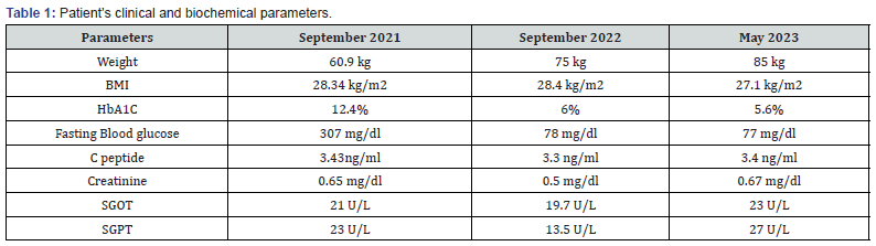
15yrs old male child was referred to the hospital with history of polyuria and polydipsia for 1 week and glycosuria. On examination acanthosis nigricans was present, his weight was 60.9kg, height 168cms and BMI 28.34kg/m2. On investigating his random blood glucose level was 470mg/dl, HbA1C 12.4%, fasting blood glucose level 307mg/dl and postprandial glucose level was 483mg/dl, blood gas study was normal. Child’s GAD65 was negative, C peptide- 3.43 ng/ml , TSH- 1.33 micro IU /ml were negative (Table 1).

His father and grandmother also have type 2 diabetes, diagnosed at the age of 35 years and 40 years respectively. Both are on oral hypoglycemic therapy and maintain normal blood glucose levels. Child was started on basal bolus regimen with insulin Degludec and insulin Lispro. His blood glucose level normalized within 2-3 weeks of starting on basal bolus regimen. He started having postprandial hypoglycemia therefore bolus insulin was stopped. Insulin requirement declined rapidly, so insulin was stopped and switched to oral hypoglycemic agent (Metformin). Genetic study was also sent. 6 months later metformin tapered gradually and stopped because of persistent low postprandial glucose level levels. Genetic sequencing reported a heterozygous missense mutation in exon 2 of NEUROD1 gene with autosomal dominant inheritance. He had no other clinical features associated with NEUROD1 gene mutation. On regular follow up his cardiac evaluation and neurological examination remained normal, and he is maintaining normal blood glucose level with HbA1C value of 5.6%. Liver function test, renal function test and C-peptide were normal.

Discussion

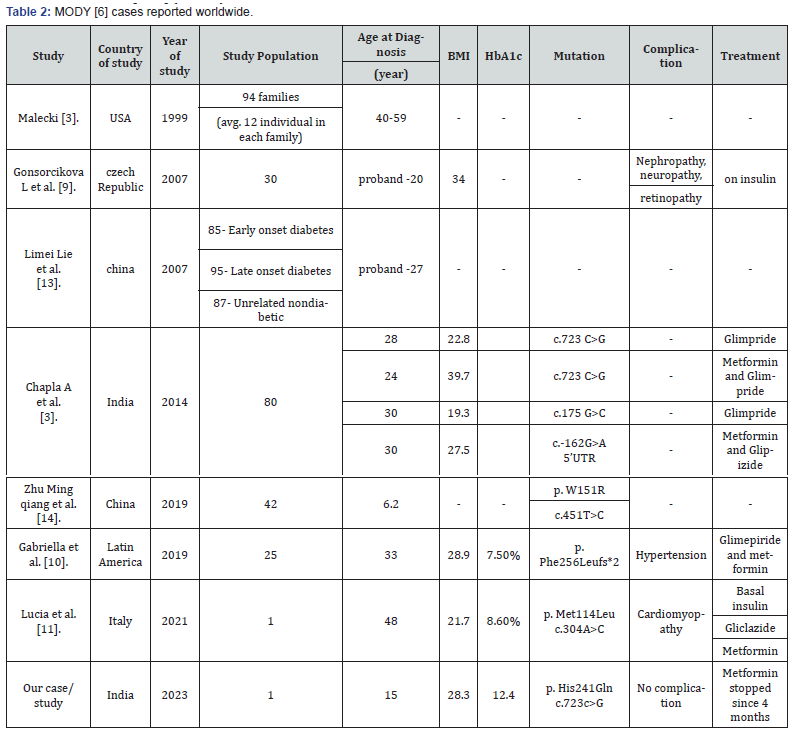
MODY: Is monogenic diabetes which is inherited in families and the common presentation is hyperglycemia which may or may not be associated with diabetic ketoacidosis. Based on the underlying mutation it is classified into 11 subtypes. The first to report association between NEUROD1 mutation and type 2 diabetes was done by Malecki et al. [3]. In 1999. With the advent of newer technologies in genetic testing, reporting of MODY6 has increased worldwide [9-14] (Table 2).

Majority of reported cases of MODY6 were diagnosed between 30 - 40years of age, mostly misdiagnosed as other types of diabetes, we are reporting one of the youngest cases diagnosed with MODY6 at 15 years of age with NEUROD1, p. his241Gln c.723 C>G heterozygous mutation. Gonosorcikova et al. [9]. reported nephropathy, neuropathy, and retinopathy as complications of MODY6. Gabriella et al. [10]. reported hypertension and one of recent study by Lucia et al. [11]. published a case of NEUROD1 who developed cardiomyopathy. Our patient had no known associated complication of MODY6 till the most recent follow up.

Aaron C et al. [12]. from India reported 4 patients with NEUROD1 mutation, between the age group of 25-30 years and all of them were on one or more oral hypoglycemic drug treatment. Patients with MODY require sulfonylureas to maintain normal blood glucose level but our case is maintaining blood glucose level in normal range without any medications, which has not been reported previously.

Conclusion

MODY should be suspected in Cases with Hyperglycemia; negative antibodies and strong family history and genetic testing should be undertaken in these cases as the most cases respond to oral medications than insulin. There are very few cases of MODY1 cases especially with NEUROD1 mutation reported worldwide, and more data needs to be available to understand the course of the disease.

To Know more about Current Research in Diabetes & Obesity Journal
Click here: https://juniperpublishers.com/crdoj/index.php

To Know more about our Juniper Publishers

Click here: https://juniperpublishers.com/index.php

Patterns of Currents in the South Euboean Bay under Variable Wind Forcing - Juniper Publishers

 Oceanography & Fisheries Open Access Journal - Juniper Publishers

Abstract

In this paper, the general behaviour of the marine circulation (sea currents) and the resulting patterns caused by wind action in the central part of the South Euboean Gulf is studied using a three-dimensional hydrodynamic model (ELCOM). The work was part of a study effort to exploit the fresh water jets that spring from the bottom of the sea, off the port of Eretria (these underwater karstic springs in the sea are called anavalos in Greek). The specific objectives were to determine the shape of the depth-averaged currents resulting from typical wind conditions and to estimate the typical time of adaptation of currents to changes in wind conditions. The South Euboean Gulf is a relatively narrow strait formed between Attica and the southernmost part of the NE coast of Central Greece, with only its central part having a considerable width, and extends for about 55 nautical miles from southeast to northwest. For the bathymetry a variable grid was used and the model was put to run simulations for each of the eight primary wind directions, for a time period of three consecutive days and then pause abruptly. The simulation period extended to seven days so as to consider the times of adaptation. No stratification was considered. The results seem very plausible and indeed are confirmed by dimensional analysis that is included in this paper as an appendix.

Keywords: Wind induced sea currents; South Euboean Gulf; Greece; ELCOM model

Introduction

The Euboean Gulf has been a subject of scientific inquiry from the days of the ancients Greeks, due to the very strong tidal effect that characterizes the strait of Euripus, near the city of Chalkis. The strait is subject to strong tidal currents which reverse direction approximately four times a day. Although tidal flows are very weak in the Eastern Mediterranean, this strait is an exception. Amongst the early scholars who studied the phenomenon we find Eratosthenes, Pitheas, Posidonios, Stravon and Senekas. There is even a tradition that Aristotle committed suicide by falling into the waters of Euripus, because he could not solve the problem, saying the famous "Since thou did not send Euripon to Aristotle, thou sent Aristotle to Euripus". This is a myth of course, because Aristotle died in Chalkis, but he died a natural death. The Gulf has been the subject of a number of studies also from the early 20^th century. Forel, the ‘father’ of Limnology, was one of the first to suggest an explanation, but a more complete analysis was presented by Aiginitis, director of the Athens Observatory, who published his conclusions in 1929.

The shape of the Gulf, and especially its southern part, south of Chalkis, being effectively an enclosed sea water body with very specific boundary conditions to its Northern end, lends itself to hydrodynamic modelling. The first hydrodynamic model for the whole of the Gulf (both its Northern and its Southern part) was constructed by Livieratos, while Tsimplis applied two models, a low resolution one for the propagation of tidal waves in the northern and southern Euboean Gulf and a high resolution one, focused on the Gulf’s Straits. Tsirogiannis et al. simulated the whole of the Euboean Gulf using the ELCOM model with important findings [1].

It is important to understand the physical processes and mean circulation patterns since they provide an indication of transport pathways of nutrients, contaminants and sediment (suspended particles). To this end, 3‐D coastal ocean models have been developed by various researchers and Universities, like for instance Princeton Ocean Model (POM), which is considered one of the first. One such model is ELCOM that solves the hydrodynamic and the continuity equations assuming hydrostatic conditions and the Boussinesq assumptions. ELCOM (Estuary, Lake and Coastal Ocean Model) [2] has been developed by CRW (Center for Water Research, University of Western Australia), and has been used extensively over the last 15 years in simulating marine and coastal ocean environments, lakes [3-5], river plume dynamics [6] and even stabilization ponds systems [7]. Modeled and simulated processes include baroclinic and barotropic responses, rotational effects, tidal forcing, wind stress, surface thermal forcing, inflows, outflows, and transport of salt, heat and passive scalars [7]. It is worth noting that ELCOM usually requires minor calibration adjustments, since the variation of most of its parameters is well defined by the conservation equations of mass, momentum and energy containing few adjustable coefficients, unlike its coupled model CAEDYM, dedicated to water quality simulation, that appears more sensitive to field data [5].

This study can be thought of as a numerical experiment or investigation, in the sense that no measured/observed field data were used for the simulations or the validation. The meteorological forcing was represented by a seasonal average for the seven days that each of the eight simulations was performed-one for every wind direction. The purpose was to determine the shape and magnitude not only of the surface currents, but also the bottom and depth-averaged circulation resulting from typical wind conditions.

Materials and Methods

Study Area

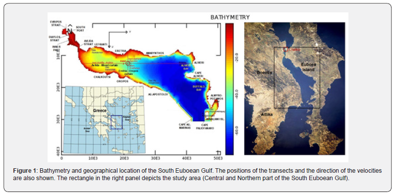
The South Euboean Gulf is formed between the eastern coast of Attica (southwards) and the southernmost part of the NE coast of Central Greece (northwards) which form its south-western shores and the southernmost part of the SW coast of the island of Evia which form its NW shores. This rather narrow and elongated sea area extends for about 55 nautical miles from southeast to northwest and is divided into three distinct parts: The Gulf of Petalia or outer part, the central part and the innermost point of South Euboean which in turn consists of the inner (northwest) part, the Strait of Diaylos and the South Port of Chalkida [8].

The central part of the South Euboean Gulf (Figure 1), which is the study area, has the southeastern boundary of Akra (=cape) Paliofanaro of the Kavalliani Island, the southwestern boundary of Akra Agia Marina and the northwestern boundary of Akra Avlidos, about 24 miles northwest of Akra Agia Marina, while the northeastern boundary is Akra Bourtzi, which is located at the same distance northwest of Akra Paliofanaro. This section extends for about 25 miles (46.3 km) from SE to NW and its width, around its middle, is 8 miles (14.8 km). The southern entrance (Kavaliani) of the central part is 1.4 miles (2.59 km) wide, while the northern entrance (Avlida) is 3/10 of a mile (0.55 km) wide and is the narrowest point of the strait of the same name (Avlida-Bourtzi). The extent of the sea area of the central part is about 460 km2 and the perimeter is roughly 160 km.

The sea depths at the southern entrance are about 70m in the middle of the distance between Isl. Kavaliani and Akra Agia Marina, while along the axis of the Avlida Strait the depths range from 8 to 14 m. The bathymetry of the bay reveals the existence of a steep slope in the direction west to east where a difference in depth of about 25 m is observed over a length of about 10 km (from the middle of the distance between Eretria and Amarynthos to the coast of Amarynthos). This slope can be said to divide the bay into a deep eastern part (east of Amarynthos) with an average depth of 53m, and a shallow western part (west of Eretria) with an average depth of 23m. The depths in the cove (inner part and South Port of Chalkis) are much shallower with a maximum depth of 10 m.

The prevailing winds according to the wind data of the Chalkida meteorological station are the North (23.4%), the Northeast (21.7%) and the Northwest (17.9%). The other winds occur with relatively low frequency (5÷7%), except for the West winds which occur relatively more frequently than the others (8.1%) [8]. Cloudiness occurs 5% of the time

ELCOM model and set-up

For the numerical simulation, as earlier mentioned, the ELCOM (Estuary, Lake and Coastal Ocean Model) model was used, a 3D finite-difference model suitable for simulations in lakes and enclosed water bodies. The main equations are the Reynolds averaged Navier-Stokes (RANS) equations using the Coriolis term, following the Boussinesq approximation and ignoring non-hydrostatic pressure terms. For the turbulence, as far as the horizontal is concerned, a constant eddy viscosity coefficient is used, while for the vertical the coefficient is obtained as a function of a local Richardson number. The density is calculated as a function of temperature and salinity according to the UNESCO equation [2].

The bathymetry was derived from digitizing the map of the Hydrographic Service of the Navy. The horizontal resolution was 200x200 m in the largest part of the field, while in parts of the field cells of other dimensions were used (non-uniform grid) in order to represent dimensions smaller than 200 m (such as the Euripus Strait). The total number of surface cells was 11,565. The following surface-to-bottom resolution was used for the vertical: 0.5 +0.5 +0.7 +0.8 +1.3 +1.7 +2 +2.5 +2.5 +2.5 +5 +7 +8 +10 +10 +10 +10 = 75m. The total number of computational cells was 162,565. A constant and uniform sea temperature of 17ºC (late autumn - spring), and a constant wind speed of 7 m s^-1 (4 Beufort) was assumed. In the northern and southern boundaries of the computational domain, an “open” boundary condition was applied, which passively allowed the water inflow to, or outflow from each cell, according to the corresponding flow needs.

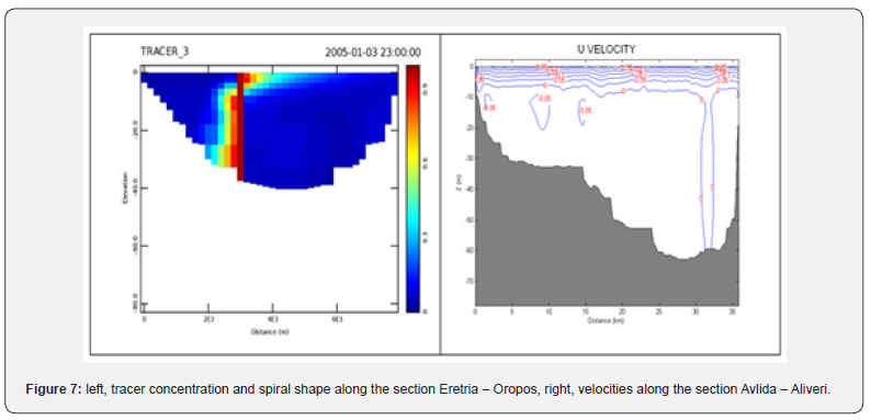
The time step was 30 sec. and the duration of the simulation was 7 days for each of the eight winds. The wind blew continuously for the first 3 days and stopped abruptly at the beginning of the fourth day. Both the dimensional analysis and the results of the simulations showed that this time period was sufficient for the flows to stabilize at the end of the third day (in fact in a much shorter time). The inertial oscillations that followed the wind cessation, however, generally did not seem to fully damp out over the next 4 days. For the visualization of the results, the model allows the creation of “curtains” i.e. sections of the water body along given lines, as well as three types of plan views or “sheets”: the surface layer (top), the bottom layer (bottom) and finally the average layer (average), which is the depth-integrated result of the parameter of interest. We used two perpendicular 'curtains' (Figure 1) at the intersection of which the position of the Eretria’s anavalos is roughly located. These curtains are a) Eretria - Oropos and b) Avlida - Aliveri. It should be emphasized here, for the sake of understanding the diagrams that follow, that the speed U increases downwards, while the speed V increases to the right. Thus, V is perpendicular to the curtain of Eretria (with positive values meaning flow towards Aliveri), while U is perpendicular to the curtain of Avlida (with positive values meaning flow towards Oropos). Finally, a tracer (Tracer_3, Figure 1) at the intersection of the two curtains was used to visualize circulation at this location.

Results

Below we will describe the actual three-dimensional circulation patterns resulting from the wind blowing for a long time from a given direction. We are going to consider winds in pairs in order to avoid confusion from the many cases.

North - Northeastern wind

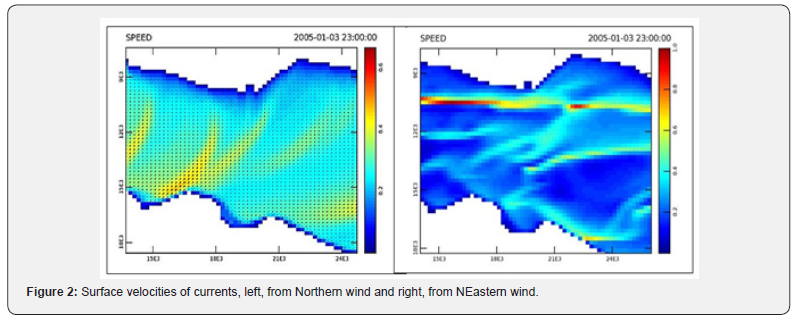
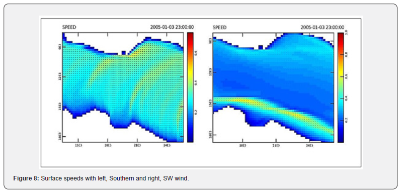
On the surface, the Northern wind breeze causes 'gusts', i.e. areas of confluence of relatively strong currents in a SW direction, while offshore, i.e. towards the Gulf of Aliveri, they take a more Western direction, as the Figure 2 shows. The northeast wind blast causes stronger currents with a westerly direction. A strong 'gust' passes off Eretria, with speeds up to 1m/s. However, it should be mentioned that of the 8 winds simulated, NE appeared unstable, i.e. the equilibrium state at the end of the adjustment time was not evident.

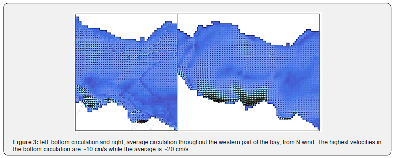
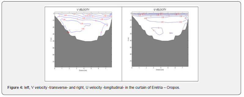
The circulation on the seabed created by the Northern wind is generally directed E and NE except for the bay of Chalkoutsi where the seabed flows 'turn' to NW (Figure 3). The resulting average circulation, as shown in Figure 3, is a cyclonic gyre with higher average speeds on the southern coast (Oropos and Chalkoutsi). We can observe this pattern also in the Eretria curtain with lines of equal V velocities in Figure 4.

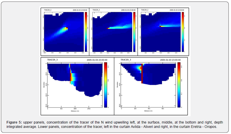
As one can see in Figure 4, the transport to Avlida takes place on the surface, while deeper there is transport to Oropos. Positive velocities - towards Aliveri - are found throughout the central part at depths below 10 m and mainly in the deeper parts of Eretria. Velocities here reach and exceed 5 cm/s. Figure 4 on the right is more difficult to read as the U velocity is parallel to the axis of the plot. However, a surface layer of about 5 m thickness with transport towards the Oropos and velocities at the surface of ~20 cm/s is shown here, while deeper in the Oropos a return current with velocities of ~5 cm/s is shown which occurs at a depth of 6 to 13 m. The total transport that takes place in the region can also be visualized using the tracer, and is shown in Figure 5. As we can see, the current generated at the surface is 45 degrees to the right of the wind, while at the bottom it is 90 degrees to the left. The average transport is almost similar to the bottom transport indicating that the main transport occurs with the bottom Ekman layer rather than the surface layer. The shape of the spiral is shown in Figure 5 below which is the Avlida-Aliveri curtain.

Western – Northwestern wind

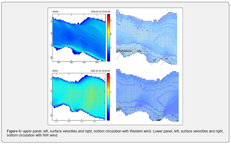
On the surface, the westerly wind creates strong surface currents along the southern coasts (Dilesi - Chalkoutsi - Oropos - Ag. Marina). The NW wind breeze creates a nearly homogeneous surface velocity field with a N to S direction (Figure 6).

On the bottom, with a westerly wind, we have a reverse flow to the W and NW in the centre of the bay and near Eretria, while on the southern coast we have the same flow as the surface flow. The average transport occurs on the North and South coasts towards E and SE with a small return flow in the centre of the bay. Overtopping is observed on the W oriented coasts. With a NW wind, the velocities in the bottom layer shift to the north. The free surface level is lowered in the interior of the bay. The surface speed of the current is at 45 degrees to the right of the wind. The bottom velocity as well as the average is again at 90 degrees to the left of the wind.

The NW wind circulation on the surface is therefore towards Oropos, while in deeper parts of the bay is towards Eretria. This is illustrated in Figure 7 where in the surface layer of about 10 m thickness the transport is towards Oropos, while below this depth there is a weak flow in the opposite direction, with higher velocities ~5cm/s, in the layer from 10 to 20 m depth, and mainly within the shallow part of the bay.

Southern - Southwestern wind

At the surface the southern wind creates currents with a Northeastern direction. The Southwestern wind creates strong currents on the northern but mainly on the southern coast of the bay.

To the south, there is a set-up on the north coast with a SW orientation. The bottom circulation is mainly to the north coast in an easterly direction and on the south coast to a westerly direction. The average circulation is very similar to the bottom circulation. With Southwestern wind there is there is a set-up on the coast with a western orientation (Buffalo Bay). On the bottom we have a reverse direction mainly in the centre of the bay while on the North and South coasts we have an Eastern direction. The average circulation is again similar to the bottom circulation.

Eastern - Southeastern wind

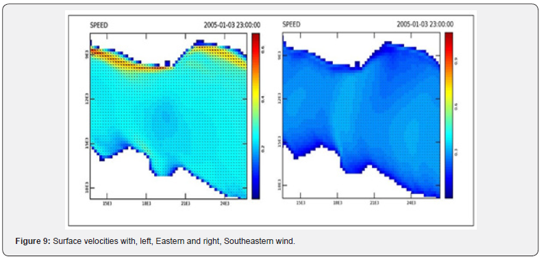
At the surface, the easterly wind creates straight currents along the Northern shores in W and NW direction. The southeast wind creates a nearly uniform velocity field on the surface in a northerly direction. The Eastern wind creates currents on the North coast of approximately the same direction as the surface currents. There is a return to the East parallel to the south coast. With a southeasterly wind the bottom circulation is the reverse of the surface circulation, i.e. to the south. On the south coast it turns to the west.

Discussion

This modeling study aimed at recognizing and quantifying the patterns of the sea currents induced by wind forcing and the resulting circulation. 3D simulations with ELCOM provide a host of possibilities for physical investigation in simulating both real time, short-term, complex marine processes but also in simulating medium and long term processes. Although the main processes can be hypothesized from theory and accumulated experience, the quantification and magnitude of the phenomena is greatly enabled by the application of the 3D hydrodynamic and thermodynamic models. In general, the application of such models in various coastal and estuary environments for a variety of purposes has been proven to be not only plausible but accurate as well [9]. The focus each time depends on the purpose and scope of the research, but there always seem to be some unpredicted -or unthought of- findings.

One such finding of the current study is that all 3 Northern winds, that prevail in the study area occurring more than 63% of the time, and with higher intensities, induce a transport of finer bottom sediment from the shores of Attica to the shallower western part of the Gulf, and partially to the across shores of Evia on a never stopping ‘conveyor belt’. The basin bed layer of the southern Euboean Gulf consists of Holocene sediments that might extend to a thickness of 14 m, while the sea bottom is dominated by mud except for the shallow coastal areas, where the sand may reach up to 50% of its overall consistency [1]. According to published maps regarding the state of the shores in Greece the western shores of Euboea appear stable, contrary to the opposite shores of Attica that experience erosion. This finding remains to be studied further and proven, or unproven, but it exemplifies the capacity of the 3D hydrodynamic models to study and model marine sediment transport issues, albeit indirectly.

Conclusion

In all cases the average transport due to the generated currents is at 90º to the left of the wind vector, i.e. that of the Ekman bottom layer. The prevailing northern winds induce a gyre that carries finer bottom sediment from the shores of East Attica to the shallower part of the Gulf, towards Avlida, and partly to the shores of Euboea. The generated currents at the surface have velocities that vary depending on the wind direction and range from 20÷60 cm/s. At the bottom, compensatory currents develop with velocities of up to 5 cm/s. The adaptation of the sea circulation (the equilibrium state) to the surface due to the wind blast occurs in about 18-24 hours from the beginning of the episode. The bottom circulation seems to reach equilibrium earlier, at 10-14 hours. The cessation of the wind is followed by inertial oscillations that fully decay in about 5 days. The latter results are further supported by the analysis in the appendix.

Appendix: estimation of temporal and spatial scales [10]

Although numerical model simulation can extend and quantify our knowledge of the hydrodynamics of a marine region, the main physical processes must be known in advance. One of the reasons why this pre-estimation is necessary is the selection and tuning of the model. We will therefore attempt below to make an assessment of the main scales, both temporal and spatial, that characterize the marine circulation phenomena in the central part of the South Euboean Gulf.

The Coriolis effect

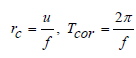
The Coriolis 'force', as we know, is the result of the rotation of the earth and causes the movements to be deflected to the right (left) in the northern (southern) hemisphere. We can weight this effect using the inertial radius r_c and the inertial period T_cor.

where f is the Coriolis parameter (f = 2Ωsinφ, Ω is the rotational speed of the Earth, Ω ≈ 7.2921*10^-5 rad s^-1 and φ is the latitude of the place, f = 8.9789*10^-5 for latitude φ = 38º) and u (ms^-1) is the speed of motion.

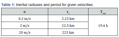
If the event in question (current motion, long-wave passage, etc.) is of a time period sufficiently shorter than T_cor, then there is 'not enough time' to deflect the direction of motion, while if the size of the basin is sufficiently smaller than r_c then the Coriolis force 'does not have enough space' to turn the velocity vector. In the case under consideration we have the following magnitudes:

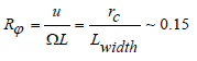
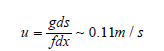
From the above table (Table 1) we conclude that for speeds such as those of sea currents (~0.2 m s^-1) there will be a significant effect of the Coriolis force, as the width of the basin (L_width ~ 15 km) is much larger than r_c, while for speeds such as that of a long wave (u = [gh]^1/2 ~ 20 ms^-1) there is no Coriolis effect.

The Rossby number, R_φ, expresses the ratio of the translational accelerations to the Coriolis accelerations, (which should be of the order of 0.1 or less for there to be a significant Coriolis effect) and the appropriate length, L, is the width L_width of the basin

Ekman Currents

The estimation of the velocities and shape of sea currents caused by the wind blast can be done by Ekman's (1905) theory. This theory describes the currents in the upper layers of the sea in equilibrium under the influence of the wind shear stress and friction of the water layers during their movement, the Coriolis force, and the local pressure gradient (the slope of the water surface). The amount of motion is transmitted from the surface to the deeper layers through vertical turbulent mixing (eddy viscosity) with a constant (according to Ekman) coefficient K_z.

As is well known, the direction of the surface current forms a 45 degree angle to the right of the wind direction (in the northern hemisphere) and its speed (which at the surface is U_E) decreases exponentially with depth. At depth z = h_E the current direction turns in the opposite direction to that at the surface and the water velocity at this depth has decreased by exp(-π), at a rate of about 4.3% relative to the velocity at the surface U_E.

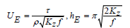
This form is called the Ekman spiral. The main transport of water due to the current occurs at a depth z = h_E /2 and is at an angle of 90 degrees to the right of the wind direction. Before establishing a free surface slope and at times shorter than the adjustment times (which we will discuss later) the sizes mentioned above are given by the following formula:

Where τ is the wind stress (Pa), ρ is the density of seawater (= 1027 kg m^-3), Kz (m² s^-1) is the constant eddy viscocity coefficient. The wind tension τ depends on a coefficient C (Ekman used the value C = 0.0026), the air density ρ_a, ρ_a = 1.25 kg m^-3, and U10 (m s^-1) the air speed at a height of 10 m above the sea surface.

So, for a typical value of K_z = 10^-3 m² s^-1

From the literature, Ekman used the following formulas

for U_E10 = 10m/s

Observations and measurements since then have finally given a surface velocity equal to half that predicted by Ekman, while the thickness of the layer was measured in very good agreement with its predicted value. At the bottom, if there is some motion, an Ekman layer will also occur in reverse order to the surface layer. This layer is called the Ekman bottom spiral.

Time scale of current adaptation

Due to the inertia of the water the wind will start to shape the surface currents with some delay. The Coriolis effect will become noticeable after t > 0.25/f ~ 46 min. The adaptation period as a whole can be approximated as

where H may be the average depth of the basin assuming that the basin is fully mixed. If we assume H = 44m and K_z = 10^-3 m² s^-1 we have T = 2.5 days approximately, while with K_z = 10^-4 m² s^-1 we have T = 7.8 days approximately.

Stream structure in equilibrium

In closed basins the prolonged wind blow will create an elevation of the water surface in the downwind direction (wind set-up). Since this will create a pressure gradient, it will also cause a compensatory flow (return flow) which takes place in the deeper layers of the basin. This circulation is complex and depends on the topography of the seabed, possible stratification, wind conditions, etc. This flow will be generated within a long-wave travel time, i.e. within about 10 minutes for a distance such as that between Eretria and Oropos (L/u =7500/17=7.3 min).

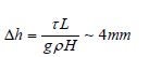
An estimate of the level difference Δh in the direction Eretria - Oropos is

with H=30m, L=7500 m and τ = 0.162 Pa.

For an estimate of the velocity resulting from this level difference

which is however considered to overestimate the actual velocity since it does not take into account the friction on the bottom.

Inertial Oscillations

If the wind suddenly deafens or changes direction then the process of adjusting the water flows under the influence of the earth's rotation to a new equilibrium state will be accompanied by oscillations around this new equilibrium position. These inertial oscillations have a characteristic period T_cor (~19h). The damping rate of these oscillations depends on their inertial period. The time scale of the adjustment of the currents to a new pressure gradient is t >> 1/f ~ 3 h. A good approximation is t~3÷5 T_cor, i.e. t ~ 2.3 to 4 days. For an estimate of the minimum adaptation time we can consider half the period of the single-node oscillation (seiche, see below).

It should be stressed that in case the basin depth is greater than hE a distinction between the two time scales should be made in order to adapt the currents to the surface layer. These time scales correspond to

a) Ekman adjustment due to Coriolis and frictional stresses in the Ekman layer

b) Inertial motion due to Coriolis and pressure gradients

It should also be mentioned that in case the wind stops we will have the creation of standing waves (seiches) in the basin (if it is closed). The period of these standing waves is given by Merian's formula:

where n is the number of nodes in the oscillation. For a single-node (n=1) oscillation we have T_h = 12.6 min for the route Eretria - Oropos.

To Know More About Juniper Online Journal Material Science Please click on:
https://juniperpublishers.com/jojms/index.php

For more Open Access Journals in Juniper Publishers please click on:
https://juniperpublishers.com/index.php

Role of Cardiovascular Magnetic Resonance Imaging in Early Detection of Myocarditis in Patients Recovered from COVID-19 - Juniper Publishers

 Cardiology & Cardiovascular Therapy - Juniper Publishers

Abstract

Objective: To assess cardiac involvement in patients recovered from COVID-19 with no clinical evidence of myocarditis, using various non-invasive parameters including Transthoracic Two-dimensional Speckle Tracking Echocardiography (STE) and cardiac magnetic resonance imaging (CMR).
Methods: This prospective study was conducted in the Cardiology Departments of Maadi Military Hospital and Benha University Hospitals. A total of 74 patients were initially enrolled during their hospital stay, but only 50 of them met the inclusion and exclusion criteria. The CMR examination was performed in conjunction with echocardiography, ECG, and laboratory investigations on the same day, which occurred 2-12 weeks after recovering from confirmed COVID-19 infection. Patient scheduling for CMR and other examinations depended on the availability of the CMR machine.
Results: According to CMR diagnosis, 23 (46%) patients were diagnosed to have myocarditis by CMR, the patients were categorized into two groups based on these results: normal group (27 patients) & myocarditis group (23 patients). According to GLS, 21 (42%) patients were diagnosed to have myocarditis by STE (diagnosis of Myocarditis with Global longitudinal strain was considered with cut-off point of >-21.33 with Sensitivity of 91.30% and Specificity of 92.59% (P <0.0001). 2D STE showed 87.50% sensitivity, 92.31% specificity and 90.00% accuracy to diagnose myocarditis, while CMR showed a 95.83% sensitivity, 96.15% specificity of and 96.00% accuracy.
Conclusion: Myocarditis was found in 46% of asymptomatic COVID-19-recovered patients. CMR is a valuable tool for early myocarditis detection when combined with 2D STE, offering high accuracy. Significant differences were observed between suspected myocarditis patients and those with normal results on both 2D STE and CMR.

Keywords:CMR; 2D STE; Myocarditis; Post COVID-19

Introduction

COVID-19 is a contagious illness caused by the SARS-CoV-2 virus, which was initially identified in Wuhan, China, in December 2019 and subsequently spread worldwide [1].

The COVID-19 pandemic has had far-reaching effects on global health, society, and economies [2]. The primary target of COVID-19 is the lungs, as the SARS-CoV-2 virus invades pulmonary tissue through the angiotensin-converting enzyme 2 (ACE2) receptor [3].

ACE2 is not limited to the pulmonary system but is also found in various other organs, including the cardiovascular system [4]. There is evidence linking COVID-19 to various cardiovascular complications, such as arrhythmias, myocarditis, acute coronary syndrome, acute onset heart failure, and cardiac arrest. Additionally, a strong association has been observed between acute cardiac injury and increased mortality rates among COVID-19 patients [3].

Previous research has indicated that a significant proportion of COVID-19 patients, ranging from 12% to 15%, exhibit elevated levels of high-sensitive cardiac troponin I (hs-cTnI) during their hospitalization, indicating myocardial injury. Furthermore, severe cases of COVID-19 may have cardiac involvement in as many as 31% of patients, but it remains uncertain how long this cardiac involvement persists after recovery [5,6].

SARS-CoV-2 has the potential to induce the release of chemokines and cytokines, which can lead to vascular inflammation, destabilization of atherosclerotic plaques, and myocardial inflammation. Consequently, elevated troponin levels in these patients could be attributed to stress cardiomyopathy, microvascular thrombosis, demand ischemia, and the secondary effects of systemic inflammation. Another possible cause of myocardial damage associated with COVID-19 is direct viral infection of the myocardium, potentially indicating viral myocarditis. While myocarditis-like clinical presentations have been reported in a small number of COVID- 19 patients, suggesting that fulminant myocarditis is uncommon [7].

Cardiovascular magnetic resonance (CMR) has emerged as the preferred non-invasive imaging technique for assessing heart volume, function, and myocardial tissue characteristics in cardiovascular medicine. Abnormalities in cardiac magnetic resonance (CMR) related to COVID-19 have been identified in 78% of predominantly ambulatory adults [8].

The main aim of our investigation was to evaluate the degree of cardiac engagement in individuals who have recuperated from COVID-19. We achieved this by employing cardiac CMR as a highly sensitive imaging method and comparing it to Transthoracic Echocardiography with 2D STE.

Patients and Methods

This prospective study was done in cardiology department of Maadi Military hospital & Benha University hospitals over 74 patients who were enrolled for this study during their hospital stay. Only 50 patients were fulfilling the inclusion and exclusion criteria and were enrolled in the study after 2-12 weeks after discharge from hospital with diagnosis of (SARS-CoV-2) by PCR on swab test of the upper respiratory tract.

The Banha Faculty of Medicine Human Research Ethics Committee approved the study protocol, and informed consent were obtained from Benha University prior starting data collection. This study was conducted over a 1-year duration, spanning from January 2021 to January 2022.

Inclusion criteria

Patients who previously confirmed with SARS-CoV-2 infection using (RT-PCR) swab test (who needs hospital admission due to significant lung affection or decreased oxygen saturation > 90%) and considered recovered by the discharging criteria ( resolved respiratory symptoms, normal temperature lasting longer than 3 days, 2 consecutive negative RT-PCR test results separated by at least 24 h and substantially improved exudative lesions on chest CT images) and were isolated for two weeks and have no any cardiac symptoms. All patients agreed to participate and sign informed consent.

Exclusion criteria were active Covid-19 infection. Previous myocardial infarction or coronary artery disease (evidence of coronary artery stenosis > 50%) , history of ischemic heart disease, previous myocarditis or heart failure, or known cardiomyopathy, uncontrolled hypertension, extremely irregular heart rates or previous atrial fibrillation, moderate to severe valvular heart disease, inability to effectively take part in breath-holding procedures and is thus unsuitable for undergoing CMR assessment, intra-cardiac devices non-MRI compatible (ICDs– Pacemakers), significant renal impairment ((CrCl rate < 30 mL/min/1.73 m2), contraindications to gadolinium contrast, disagree to participate or sign informed consent and insufficient CMR image quality for analysis.

All cases underwent a full history taking, complete physical examination, 12 leads Electrocardiogram, laboratory investigations (Creatinine, Troponin I & CBC), trans-Thoracic Echocardiography which was done for all patients according to EACVI Echocardiography guidelines [9] (Conventional study & 2D Speckle tracking), and CMR.

Protocol for CMR scanning included the following

conventional sequences: long-axis and short-axis cine, late gadolinium enhancement (LGE) and T2- weighted imaging (T2WI).

Quantitative mapping sequences: post-contrast T1 mapping and native T1/T2 mapping.

The diagnosis of myocarditis was confirmed by Updated Lake Louis criteria (2018) for diagnosis of Myocarditis which consist of two main criteria (T1-based criterion and T2-based criterion). The T1-based criteria is regarded as positive when there are increases in native T1 relaxation durations, increases in extracellular volume (ECV), or the presence of positive LGE.

The T2-based criterion is positive when there is an increase in T2 relaxation times, regionally high T2 signal intensities on T2- weighted images, or an elevation in the global T2-signal intensity ratio.

Supportive Criteria: pericardial effusion, pericardial signal abnormality, systolic LV dysfunction. All CMR images were evaluated by consultant cardiologist with 6 years of CMR diagnosis experience.

Sample size

Using PASS software, the minimum sample size required for specificity and sensitivity tests was calculated (PASS 11 citation: Hintze J (2011). PASS 11. NCSS, LLC. Kaysville, Utah, USA). The required sample size for the study is determined to be 50 patients without accounting for dropout rate.

Statistical Analysis

We conducted the statistical analyses using SPSS software (Statistical Package for the Social Sciences, version 24, SSPS Inc, Chicago, IL, USA). Categorical variables were presented in frequency tables with corresponding percentages, whereas descriptive statistics like standard deviation and mean were used to describe numerical data. Data entry, processing, and statistical analysis were performed using MedCalc ver. 20 (MedCalc, Ostend, Belgium). We employed various tests of significance, including logistic multiple regression analysis and ROC Curve analysis. The choice of analysis method was based on the nature of the data, whether it was parametric or non-parametric. We considered p-values less than 0.05 (5%) to be indicative of statistical significance [10].

Results

Table 1 shows demographic data, risk factors and vital signs in all studied group. Table 2 shows ECG data, lab investigations, 2D speckle tracking Echocardiographic parameters and diagnosed myocarditis by CMR in all studied group.

BMI: body mass index, HTN: hypertension, DM: diabetes mellitus, HR: heart rate, SBP: systolic blood pressure, DBP: diastolic blood pressure, MAP: Mean Arterial pressure.

EF: Ejection Fraction, LVESD: Left Ventricular End-Systolic Dimension, LVEDD: Left Ventricular End-Diastolic Dimension, LAD: Left Atrial Dimension, TAPSE: Tricuspid Annular Plane Systolic Excursion.

According to CMR diagnosis, 23 (46%) patient was diagnosed to have Myocarditis by CMR using Updated Lake Louis criteria (2018) and patients were categorized into two groups based on these observations: normal group (27) patients & myocarditis group (23) patients.

There was no statistically significant difference between both groups regarding age, sex, BMI, SBP and MAP. While the HR, DBP & TLC were higher in myocarditis group than in normal group with statistically significant difference (P=0.008, p=0.006 & p= 0.001 respectively). The lymphocytic count was lower in myocarditis group with statistically significant difference (p<0.001). Table 3 A statistically significant difference was seen between the two groups regarding ECG data and Troponin I during hospital stay with higher incidence of abnormal ECG & elevated Troponin I in myocarditis group than the other group. (P<0.0001). Time interval per weeks was about 4.5 weeks between hospital discharge & CMR & Echocardiographic examination with no significant difference between both groups. Table 4 Average left ventricular (LV) systolic function in myocarditis group was significantly lower than the normal group (P <0.001). Differences between the two groups were statistically significant concerning the LVESV (P = 0.012) & the LVEDV (P = 0.002). The average right ventricular ejection fraction (RVEF) was no significant difference between both groups. Global native T1, T2 values showed significant elevation in myocarditis group compared with the normal group (P. <0.001). Global Native T2 was significant high in the myocarditis group than in the normal group (P.<0.001). Pericardial enhancement and pericardial effusion were found in 14 patients (60.8%) of myocarditis group and was absent in normal group (P. <0.001). According to 2D STE parameters, there was a statistically significant difference between both groups regarding EF (P<0.0001), LVESD (P=0.014) TAPSE (P=0.028) and LAD (P <0.0001).

*: significant P value, BMI: Body Mass Index, DM: Diabetes Mellitus, HTN: Hypertension, HR: Heart Rate, SBP: Systolic Blood Pressure, DBP: Diastolic Blood Pressure, MAP: Mean Arterial Pressure.

Global longitudinal strain was significantly lower in myocarditis group (-16.34% vs -23.07%). Also, base longitudinal strain, mid longitudinal strain and apical longitudinal strain were lower in myocarditis group (P<0.0001) (Table 5).

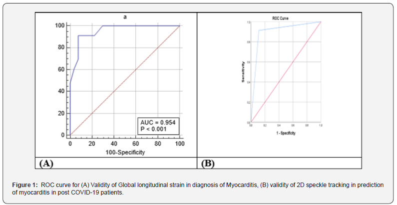
2D speckle tracking Echo parameters were used for diagnosis of myocarditis with global longitudinal strain cut-off point of >-21.33 with Sensitivity of 91.30% and Specificity of 92.59% (P <0.0001). 2D STE showed a Sensitivity of 87.50%, Specificity of 92.31% and Accuracy 90.00% for detection of myocarditis, while CMR showed a Sensitivity of 95.83%, Specificity of 96.15% and Accuracy 96.00%. Figure 1 Logistic regression analysis was conducted for the prediction of myocarditis in the studied patients. Global longitudinal strain, LVEF, LVESV, LVEDV, NativeT1, NativeT2, DBP, HR, TLC, Lymphocyte, troponin I, ECG abnormality, EF, LVESD & TAPSE were associated with the risk of myocarditis in univariate analysis. Only global longitudinal strain was associated with risk of myocarditis in both univariate and multivariate analysis Table 6.

*: significant as P-value.

*: significant as P-value, LVEF: Left Ventricular Ejection Fraction, RVEF: Right Ventricular Ejection Fraction, LVESV: Left Ventricular End-Systolic Volume, LVEDV: Left Ventricular End-Diastolic Volume, LGE: Late Gadolinium Enhancement, SIR: Signal Intensity Ratio.

Discussion

Myocarditis is a condition that results from inflammation of the heart muscle, usually caused by a viral infection or an autoimmune disease. With the outbreak of COVID-19, reports of myocarditis cases in patients who have recovered from the virus have emerged. Given the severity of the pandemic, the early detection and treatment of myocarditis are crucial to prevent longterm cardiac damage and potential complications.

The mean age in our study group was 35.5 ± 8.24 years, this was concordant with Huang et al. [11], who studied 26 patients who recovered from covid-19 and stated that patients with a mean age of 38. In contrast Wang et al. [12], who investigated cardiac consequences of COVID-19 in 47 recovered patients using CMR, reported higher mean age as they stated that mean age of their patients was 47.6 ± 13.3 years, In our study 41(82%) were males which was consistent with Ulloa et al. [13] Who studied 57 recovered patients searching for myocardial affection in recovered patients from covid-19 with male predominance with 80% of study group were males. In contrast, Huang et al. [11] showed female predominance as only 38% of study group were males.

In our study, 28 (56%) of all studied group were smokers, 13 (26%) patients had DM and 19 (38%) had hypertension. This was comparable with Wang et al. [12] Who reported that 18% of their patients had DM and 25% of them had hypertension. In contrast Huang et al. [11] in which only 8% of patients were hypertensive and none had DM..

According to CMR parameters, 23 (46%) patients were diagnosed to have myocarditis by CMR, and patients were categorized into two groups based on these results: normal group (27 patients) & myocarditis group (23 patients).

There was no statistically significant difference between both groups regarding age, sex, BMI, SBP and MAP. Differences between the two groups were statistically significant regarding DBP, HR, TLC and lymphocytic count. In contrast, Huang et al. [11] reported that there was no statistically significant difference between patients with normal and abnormal CMR finding regarding age, sex, SBP, DBP, HR, TLC and lymphocytic count.

Our study showed statistically significant difference between both groups regarding level of Tn I as we found 11 (47%) patients with elevated Tn I in myocarditis group versus only 1 (3.7%) patient in the normal group. This was in line with Wojtowicz et al. [14] who reported statistically significant difference between the two groups of patients with and without non- ischemic cardiac injury using CMR regarding Tn I level. In the current study, there was a statistically significant difference between both groups regarding ECG abnormality as we found 12 (52%) patients with ECG abnormality in myocarditis group versus only 1 (3.7%) patient in the normal group. This was supported by a study by Ulloa et al. [13] which was conducted in Spain and studied myocardial affection in post covid-19 patient over 57 patients and showed statistically significant ECG abnormality which was found in 24 post covid patients (42%) inform of RBBB (15.8%), Atrial fibrillation (5.3%), Ventricular extrasystole (1.8%), Negative precordial T wave (12.3%) and Pathological Q wave (7%).

In our study, Echocardiographic examination showed statistically significant difference between both groups regarding EF, LVESD, TAPSE and LAD. In comparison, Özer et al. [15] who studied 74 patients with previous Covid-19 infection after 1 month from recovery reported also statistically significant difference between patients with elevated troponin group and the other group without elevated troponin regarding LAD, LVEF but no statistically significant difference between both groups regarding LVESD & LVEDD.

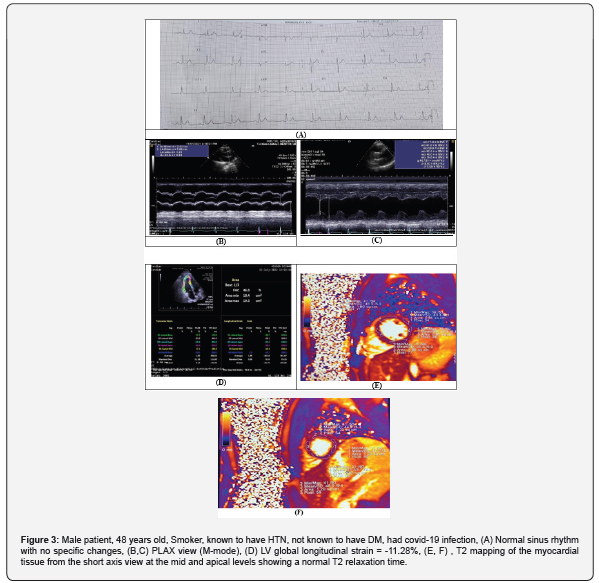
Our study found 21 (42%) recovered Covid-19 patients of all studied group had reduced GLS. This was in line with Mahajan et al. [16] who found reduced GLS in 40 (29.9%) recovered Covid-19 patients of his study group.

In our study, Global longitudinal strain was significantly lower in myocarditis group. Also, Base longitudinal strain, mid longitudinal strain and apical longitudinal strain. In line with our study, Mahajan et al. [16] showed statistically significant difference between reduced LV GLS group and Normal LV GLS group regarding LV GLS.

In contrast, Özer et al. [15] reported no statistically significant difference between group with myocardial injury and the other group without myocardial injury regarding LV GLS (-17.7 ± 2.6 Vs -18.9 ± 1.8, P=0.051). In our study we found 23 out of 50 (46%) patients had abnormal CMR parameters including myocardial oedema and LGE and diagnosed as myocarditis by updated Lake Louise criteria with mean time between hospital discharge and CMR examination of 34 days. This was in line with Huang et al. [5] who found median (IQR) time between COVID-19 diagnosis and CMR was 47 (36-58) days, and 15 of 26 patients (58%) reported abnormal CMR results on conventional CMR sequences.

In our study, myocarditis group were significantly different from healthy one in CMR examination regarding LVEF, LVESV, and LVEDV. But no statistically significant difference regarding RVEF. It was in concordance with Wojtowicz et al. [14] who reported statistically significant difference between the two groups of patients with and without Non-Ischemic Cardiac Injury regarding LVEF (57% vs 61%, P<.001), but no statistically significant difference regarding LVEDV and RVEF.

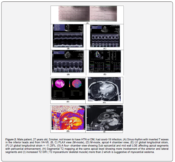
Our study showed increased myocardial oedema parameters with statistically significant difference between myocarditis and normal groups in form of increased T2 signal intensity ratio (T2 SIR), increased T2 relaxation time and increased native T1 respectively. In concordance to our study, Huang et al. [5] revealed that global native T1, T2, and ECV values were significantly greater in recovered COVID-19 patients with positive conventional CMR findings than in patients without positive findings (native T1 1,271 ms versus 1,237 ms, P=0.002), (T2 42.7± 3.1 ms vs 38.1± 2.4 ms, P=0.005), (ECV 28.2% vs 24.8%, P=0.001).

Also, Kunal et al. [17] reported significantly elevated native T1 (1301ms Vs 1264 ms, P =0.022) and native T2 (55.62 vs 45.25 ms, P =0.004) in post Covid-19 patients with abnormal CMR group compared to the other one with normal CMR.

In our study, non-ischemic pattern of LGE was found in 23 patients (46%) mainly sub- epicardial and mid wall enhancement affecting the apical and mid cardiac muscle segments with P value <0.001, denoting presence of myocardial fibrosis and/or necrosis. Wang et al. [12] reported non-ischemic sub-epicardial and mid wall LGE in 13 of 44 (30%) of the post-COVID- 19 patients’ group (a finding similar to our cohort results). Then they performed a strain study revealing that patients with LGE exhibited poorer LV and RV Performance.

In our study, Pericardial involvement in form of pericardial effusion and pericardial LGE which develops as a consequence of myocardial damage, was also found in 14 patients (28%) of all studied patients and was found in 60% of myocarditis group. In concordance, Huang et al. [5] reported that 7 (28%) of 26 patients were positive for pericardial LGE and have a minor pericardial effusion.

Regarding the validity of 2D speckle tracking Echocardiography (STE) and CMR in final diagnosis of myocarditis, In previous study by Luetkens et al. [18] found that the diagnosis of myocarditis using Updated Lake Louise Criteria yielded a sensitivity of 87.5% and a specificity of 96.2%.

In our study, speckle tracking echocardiography showed a sensitivity of 87.5% and specificity of 92.3 %. A study by Sharifkazemi et al. [19] compared the diagnostic performance of CMR and 2D STE in 57 patients with suspected acute myocarditis. They found that CMR had a higher sensitivity (96.8%) and specificity (93.5%) compared to 2D speckle tracking Echo (78.4% and 77.4%, respectively) in the diagnosis of acute myocarditis. In our study logistic regression analysis showed that only global longitudinal strain was associated with risk of myocarditis in both univariate and multivariate analysis.

Finally, this study had some limitations, as study did not include long-term follow-up to assess the outcomes of patients with myocarditis. Also, the study did not provide detailed information on the severity of COVID-19 in the patients, which may have influenced the development of myocarditis.

Case Presentations

Case 1: Figure 2. Case 2: Figure 3.

Conclusion

Evidence of myocarditis in asymptomatic patient recovered from COVID-19 was present in 46% of patients. Non-invasive predictors of myocarditis are Global longitudinal strain, LVEF, LVESV, LVEDV, NativeT1, NativeT2, DBP, HR, TLC, Lymphocyte, TnI, ECG abnormality, EF, LVESD and TAPSE while Global longitudinal strain was the only independent predictor. According to this research’s findings, it can be concluded that CMR is a valuable tool in the early detection of myocarditis in those who have achieved recovery from COVID-19. The use of CMR in combination with 2D STE has shown a notable level of accuracy in the detection and assessment of myocarditis. The findings of this study showed that there were significant differences between patients with suspected myocarditis and those with normal results on both 2D STE and CMR. The results also showed that CMR had higher sensitivity, specificity, and accuracy compared to 2D STE in the diagnosis of myocarditis. Further studies with larger sample sizes and multi-center cooperation are needed to validate the diagnostic accuracy of CMR and 2D STE in the early detection of myocarditis in patients recovered from COVID- 19.

To Know more about Journal of Cardiology & Cardiovascular Therapy

Click here: https://juniperpublishers.com/jocct/index.php

To Know more about our Juniper Publishers

Click here: https://juniperpublishers.com/index.php