Juniper Publishers

Juniper publishers have been established with the aim of spreading quality scientific information to the research community throughout the universe. We, as Open Access publishers, strive to offer the best in class online science publications. Open Access process eliminates the barriers associated with the older publication models, thus matching up with the rapidity of the twenty-first century. Our main areas of interest lie in the fields of science, engineering and other related areas.

Thursday, December 16, 2021

Line-by-Line Sweeping Method in Hydraulic Head Distribution - Juniper Publishers

Trends in Technical & Scientific Research - Juniper Publishers

Abstract

Numerical solutions have been extensively used in recent decades to solve engineering problems in different fields such as fluid dynamics, heat transfer and soil mechanics. In this study a hybrid implicit finite difference approach has been used to calculate the hydraulic water head distribution which is a combination of Gauss-Seidel and Alternating Direction Implicit method. By solving seepage equation for stable flow condition in a two-dimensional homogenous and isotropic environment, water head distribution from high to low values is calculated from four neighboring cells. Results showed by travelling from right to left in head contours, density and value increased. Water head has been divided into 12 equipotential lines. The benefit of using such numerical solutions is their high accuracy and consistency.

Keywords: Numerical Simulation; Finite difference method; Line sweeping; Hydraulic head distribution

Introduction

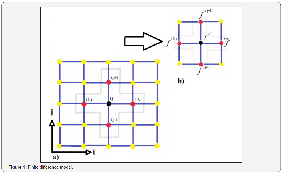
An engineering problem with too many assumptions and simple mathematical model results in analytical solution which is a good approximation to reality [1-3]. On the other hand, engineering problem with low assumptions and more complex math models ends in numerical solutions [4-7]. Numerical models are classified into three major categories. Finite difference, finite volume, and finite element modeling. Finite difference has been developed by Euler in 1768. The earliest mathematical paper describing the technique date back to Shellback’s work of 1851 [8]. One other method is finite volume method which is almost the same with finite difference method except an integration step ahead of finite difference [9-11]. From 1950 finite element method (FEM) has been developed and extensively used specifically for structural frame analysis etc. [12-14]. Any finite difference model includes two main parts. First is domain discretization which is shown in Figure 1 below. And the second component is equation discretization. Equation (1) shows a sample of equation used in finite difference method.

In discretization of equation an approximation based on teylor’s expansion has been used [15-17]. Beside, elements relation in the modeling domain has a high degree of importance. Finite difference can be used in advection-diffusion equation, conservation of mass or in solving Navier-Stokes equations both in explicit and implicit formats [18-20]. Other advantages of using numerical solutions is their consistency, stability, convergency and finally their accuracy. Courant number is responsible for stability of the model [21].

Method

Alternating direction implicit (ADI)

In this method equations are solved in a sequential order in terms of rows and columns of a matrix respectively. The whole idea is to solve the first set of equations, rows per say in first time step and the others (columns) in next time step [22,23].

Gauss-seidel method

It is an iterative method used to solve a system of linear equations which is named after the German mathematicians Carl Friedrich Gauss and Philipp Ludwig von Seidel [8]. In this iterative method equation with higher coefficient used as a base for starting equation.

Line by line sweeping method

This method is a combination of Gauss-Seidel and ADI method. By solving seepage equation for stable flow condition in a two-dimensional seepage environment we have equation (2) as below. Considering homogenous environment (K is constant in all directions) and isotropic condition (K_x = K_y) equation (2) simplified into equation (3).

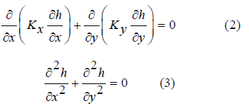
By applying second order finite difference method, equation (3) results in equation (4).

If ∆x = ∆y, then hi, j is calculated from four neighborhood cells as presented in Figure 1 as well as equation (5) below.

Boundary and initial conditions

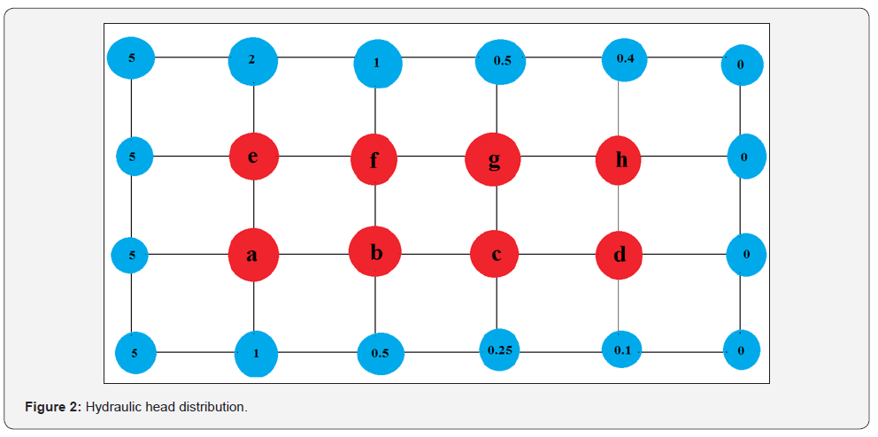
Figure 2 shows a schematic of problem. This study investigates hydraulic head distribution based on a line-by-line implicit sweeping method. A 4×6 matrix has been considered in which boundary conditions at the left and right sides as well as up and down of the domain was given as known values in blue circles in terms of meters of water head. In this study water head stands at 5 meters at the left-hand side and eventually reaches to zero at the right-hand side. Boundary conditions and their values are shown in blue circles. Calculated values are presented in central red circles having initial values of two meters of water starting from lower case e and end at lower case d.

By applying the sweeping method from second row, all red circles have been calculated from four neighboring method which has been mentioned earlier. In next step by starting from second column and having previously calculated results as initial known values for this step, values of second iteration were calculated. To check the model convergence, a convergence condition has been applied.

Successive Over Relaxation (SOR)

α = 1.5 considered as relaxation coefficient and should be higher than one.

Results

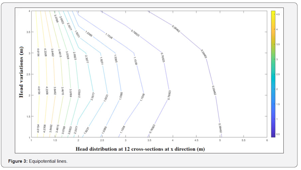
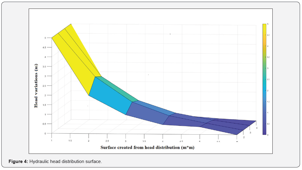
Figure 3 shows distributed head contours from high to low values. By travelling from right to left contours density and value increased. In fact, the height of five meters of water has been divided into 12 equipotential lines, in which each single line stands for a cross-sectional head at that height of water. The reason of having low congestion of equipotential lines at the right-hand side (lower head values) of Figure 3 is the mild slope of head distribution as it is presented in Figure 4, hence equipotential lines are in further distances in comparison to the left -hand side (Higher head values). Figure 4 below shows a schematic of head distribution surface.

Conclusion

In this study, with the help of a numerical approach a fluid dynamic solution has been developed for a hydraulic head distribution of water throughout a hybrid line-by-line procedure which is a derivation of Alternating Direction Implicit Method (ADI) and Gauss-Seidel method. Numerical solutions have high accuracy and consistency as well as convergency and stability. These characteristics gives us a privilege in replacing them with many analytical and traditional fluid dynamic solutions. Their accuracy leads in having less errors in our results, and their convergency ends in reaching the almost same algebraic solution results.