Robotics & Automation Engineering Journal

Nowadays many dynamic systems, both deterministic as well as stochastic by nature, have become more and more complex: nonlinearity, the influence of the time delays and time forecasting terms, etc. Applicability of such systems is widespread: system analysis of the safety problems and optimization of the diverse technical, technological, socio-economic and other processes. The concept of the complex dynamic system (CDS) and the problem of a creation and an investigation of the mathematical models of the CDS are in focus of a number of the modern scientific and engineering fields, and of the many other areas including the robotics and automation.
The basic features of the CDS, approaches for their modeling with an account of the real factors, time delays, and forecasting terms, the influence of the different possible non-linearity effects are presented and discussed. Different modeling approaches are considered and analyzed in detail together with the problem of stability and stabilization of the systems. Instability of a system may cause improper work of it or even lead to a critical regime or a total collapse of the system, which is highly important for a control. The question of an optimal control is discussed too because the modeling and controlling challenging tasks are interconnected in the CDS. Some results of the research are provided together with the examples of computer simulations. Conclusions about the results obtained and the future research directions are given.
Keywords: Modeling; Dynamic systems; Non-linearity; Time delay; Time forecasting; Critical level
Abbrevations: CDS: Complex Dynamic System; PHO: Potentially Hazardous Object; KTH: Royal Institute of Technology
Introduction
Historically probably the first investigator of the equation for system development was T.R. Malthus, English economist, statistician and demographer born at Guilford, Surrey,who already in the18th century has considered the simplest development equation in the following form[1,2]:

where у,t are the function describing the evolution of some magnitude and time, respectively, k is the growth factor of the system, which generally can be a function of time. Malthus was a pivotal figure in a development of the empirical study of the human populations who is very well known in the world for his Essay on the Principle of Population, the central theme of which was postulated inherent tendency for amount of a human population to `outstrip the means of subsistence’, based on solution of the equation (1) 0ktyye= where 0y is the initial number of the people in a population. By Maltus and his followers, a human improvement therefore depended on the stern limits on reproduction. The original essay, published anonymously in 1798, was directed against the optimistic speculations of the utopian writers believing in no limit to human progress. The solution of equation (1) for the simplest case with a constant growth rate k has shown that a law of population growth was seen as threatening to a society and spawned the philosophical course of the Malthusianism, which justified the war as a necessary mechanism for a regulation of the population’s growth. It was a big mistake based on a simplified equation of the system’s growth. In fact, later on it was shown that the system could start its development following the law (1), but further the coefficient k depends on time, e.g., decreases according the hyperbolic law (so called allometric process). Thus, the function’s increasing rate decelerates with time. Since that time, there were many attempts to use this simple equation of a development, and many others, more accurately accounting the characteristics of the systems under consideration.
An observation of a number of systems has shown the development processes better described in several other equations: over time, in some cases, coefficient k is being gradually or abruptly falling down, and this leads to solutions, in which there is no exponential growth function. This behavior corresponds better to the realities of different systems of diverse nature: first, there is an intensive development process, which is adjusted according to the results of the development and to an analysis of a development’s needs. In the real systems, some time delays and forecasting terms are met. The first ones are caused by delays in the control mechanisms, while the second ones are available due to a planning and an orientation of the control system to the desired future performance rather than to a current real state. Development of the mathematical models to analyze and simulate the different industrial, socio-economic, automated and other CDS is of interest both in a scientific, as well as in the applied aspects.
The Aggregated Mathematical Models for Computer Simulations of the Potentially Hazardous Objects
For example, the mathematical modeling and computer simulation of the potentially hazardous objects was considered in touch with a need of a tactical and strategic planning and decision making support in a lot of the environmental and other tasks to reveal and analyze the peculiarities of the real systems depending on the different delays and forecasting terms as it is normally met in a real world [3-10]. We developed and investigated the aggregate dynamical models for the potentially hazardous objects (PHO) in touch with safety estimation for the nuclear power plants and the other types of hazards [3,4,6-9].Complex systems with a large number of governing parameters and many possible delays and forecasting terms are difficult to investigate analytically but it is successfully done using the computer simulation. For example, the aggregated mathematical model of a potentially hazardous object in a nuclear power (the similar mathematical models can be also developed for some other objects) has the following form [3,7-9]:

where ij τ are the time delays for the corresponding parameters. Such indexes in a more general case also, in turn, depend on the time (and possibly each other). Here i z− - the parameters of a system, bij− coefficients of the mathematical model, which are determined for each model based on the results of its functioning using the methods of systems’ identification. The system of differential equations (2) allows analyzing the critical levels of the CDS using computer simulation methods. Some results are presented in the Figure 1-4, where from it is clearly observed that some dynamic modes can be critical and even catastrophic. Detection of the parametric dependencies and characteristics is much more complicated than the above case (1) and similar to it, where the concept of the main features is clearly understandable.


The effective numerical methods and methods of averaging the differential, integral, as well as the integro-differential operators allowing performing mathematical simulation in a wide range of complex processes and systems are applied for solution of differential equations with delayed and forecasting arguments. In particular, modeling the dynamics of the behavior of potentially hazardous industries, based on statistical information about the objects. The aggregate models for the development of nuclear energy facilities were constructed and studied [3,4,6-9]. It allowed computational experiments to identify the interesting features in the development of nuclear energy industry or an individual nuclear power plant, the optimal strategy, identification of the critical and dangerous situations, etc. To some extent, this can contribute to improving the management of the relevant objects and reduce their negative impact on the environment.
Since such complex objects in most cases do not allow constructing the precise deterministic mathematical models due to big or even huge number of influential parameters and often unknown links between them, then the aggregate model built on statistics about the object can be useful for studying the nature and behaviors of the objects. This paper focuses on the modeling and analysis of the behaviors of different systems based on the latest achievements in the theory. In particular, the method developed in the book by Zhirmunsky & Kuzmin [11] who considered a lot of different applications. The equations for the development systems with delayed and forecasting arguments have been considered in many different aspects [11-26]. It was shown, which levels must be the intensities of development and other parameters so that the system is kept in a state of stable development and not subject to the modes of oscillations growing in time by an amplitude that rapidly destroy it (instability, catastrophes, the disintegration of the system). Our study focuses on peculiarities of the systems’ behaviors in a methodological and mathematical aspect, the task of constructing and using such models of the applied nature. Also, the features of performances of a number of outstanding tasks are discussed as well.
The results of computer situational simulations in a wide range of variable parameters given the shift of the arguments enable to identify and explore some of the most important features and phenomena as an optimizing plan, and dangerous for the development and operation of the CDS. The identified critical conditions and catastrophic situations and scenarios, which for the system can get, should be carefully studied with the purpose of their conditions in a real object. Many different peculiarities of the CDS of diverse nature may be revealed through computational experiments, by numerical simulation in a wide range of parameters and conditions.
Development of the models for studying the evolution of complex systems (economic, political, social, banking, physical, combined by different nature and properties, etc.) in a rather general setting requires consideration of the delayed and forecasting temporal arguments, because development of the system is really accompanied by some delays compared to the planned indicators due to various reasons, as well as orientation for leading indicators what is known as the term “foreseen adaptation”. Such phenomena have actually been observed in a number of different processes and systems as a wildlife and technical origin.
Development of the Different Types Aggregated Mathematical Models
In general case the aggregated dynamical model of the PHO can be presented as follows [3,6,9]:

where x (t) i are the characteristic parameters for PHO, i N are the limit values of i -th parameter, a−ij the coefficients, which may be a function of time, n − the number of parameters of the PHO, i =1,2,...n . The limit values Ni may vary according to the problem stated: tactical or strategic planning, calculation of the dynamic evolution of the parameters, critical regimes of the PHO, etc. The non-linear ordinary differential equation array (1) with the corresponding initial data determines the peculiarities of evolution in time until the achievement of the planning values or any kind of other regimes, for example, saturation, critical points in the system, catastrophes, and so on.
The parameters xi can be stated as follows [6]: x1 - the quantity of the working personnel at the PHO, x2 - the quantity of the managers at the PHO, x3 - the total amount of product output at PHO, x4 - the expenditures for the repairing and restoring at PHO, x5 - the expenses required for elimination of a negative influence on the environment, x6 - the safety culture level.
The variables may change in the range from 0 to Ni ( N6 =1 is chosen just for simplicity). The first step in a development of the PHO model consists in calculation of the constants in the equation array (3) using the statistical data collected. For a lot of diverse PHO, this is a crucial problem due to absence or uncertainty of the statistical data about its functioning. Also, a serious problem is the identification of the model, which requires computing the coefficients aij from the satisfaction of the model developed with the real object.All variables of the model can be divided by their characteristic scales: yi = xi Ni ,bij = aij N j ,bi0 = ai0 , y6 = x6 . Then the equation array (3) is transformed to the following dimensionless form

which has stationary solutions, one of which is trivial when =1 i y for all values of the PHO parameters. Here the 6 variables have been stated. Actually, it may be more variables depending on the situation and existing knowledge and statistical data about the object. Coefficients aij in the equations (3) and coefficients bij in the equations (4) may be estimated by their possible signs. For example, in a first equation of (3) must be a11 ≤ 0 , a16 ≤ 0 , a1j ≥ 0, j=2-5. Here a11 ≤ 0 means that the more people are working at the PHO object, the more the first term in the first equation of (1) decreases the further growing rate of the number of workers. It may be stated that a1j ≥ 0 , (j=2-5) due to the fact that the number of managers, the quantity of the product produced at PHO, expenses on the repairing, etc. can only lead to increasing of the workers needed. Similarly a21 ≥ 0 , a23 ≥ 0, and the rest of the coefficients in the second equation of the system (3) must be negative because only the growth of the workers’ number and product may result in a request for growing the number of managers. All the other factors result in a decrease of the managers’ amount at the PHO.
In the third equation only one coefficient is supposed to be negative: a33 ≤ 0 . This is because the product amount growing causes the further productivity falling. All the other factors act to its growing. The fourth equation gives a44 ≤ 0 ,a46 ≤ 0 because the increase of all expenses tend to their decrease afterward as far they keep sufficient some time. And the increase of safety culture makes the tendency to decrease of all expenses. In the fifth equation only the last 3 coefficients seem to be negative: a5j ≤ 0 , j=4-6, where a54 ≤ 0 because by growing the expenses for the repairing of a different part of PHO there is less money going to ecology and other stuff, a55 ≤ 0 because if paid for this need, then less is going later on for this. The last equation also must contain the last three coefficients negative: a6j ≤ 0( j=4-6): the payments for the repairing and other stuff needed are directly connected to a safety culture (the higher is safety culture, the less are those expenditures required).
As clearly observed from the Figure 4 by the results of computer simulation using the mathematical model developed [3], the nonlinear system is smoothly growing starting from the appropriate initial state. The parameters of the PHO and their phase portraits (derivatives of the parameters by time depending on the phase coordinates) in Figure 4 are numbered and the initial data are given below:

(y1=1.-0.8, y2=1.-0.9, y3=1.-0.8, y4=1.-0.7, y5=1.-0.2, y6=1.- 0.5)
(xN1=50000., xN2=5000., xN3=333333., xN4=5000., xN5=5000., xN6=1.)
(A10=-0.3, A11= 1.0e-06, A12=-1.0e-05, A13=-1.0e-06, A14= 1.0e-04, A15= 1.0e-04, A16=0.)
(A20=-0.2, A21= 1.0e-06, A22=-1.0e-05, A23=-1.0e-06, A24= 1.0e-04, A25= 1.0e-04, A26=0.)
(A30=-0.1, A31=-1.0e-05, A32=-1.0e-06, A33=-1.0e-05, A34= 1.0e-04, A35= 1.0e-04, A36=-0.1)
(A40=-0.1, A41=+0.0e-00, A42=+0.0e-00, A43= 1.0e-06, A44=-1.0e-04, A45=-1.0e-04, A46=-0.3)
A50=-0.1, A51=+0.0e-00, A52=+0.0e-00, A53= 1.0e-06, A54=-1.0e-04, A55=-1.0e-04, A56=-0.3)
(A60=-0.34, A61= 1.0e-06, A62= 1.0e-05, A63= 1.0e-06, A64=+0.0e-00, A65=+0.0e-00, A66=0.).
Analysis of the computations presented in Figures 1-4 allows revealing some peculiarities of the PHO, including optimal and critical regimes. This information can be used for optimal control of the CDS’ development, e.g. functioning of the PHO of nuclear energy. In the last case, it gives the possibility to avoid some critical situation in operation of the PHO and even some potential accidents. After identification of the PHO, which consists in determining the constants of the mathematical model by comparing the computer simulations with the results of its real work, the results of computer simulations by the model developed may be used for tactic and strategic planning of the PHO functioning. For example, substantial oscillations of the phase trajectories of some parameters mean the possibility for abrupt changes in the regimes of the system’s functioning, with a comparably weak deviation of its parameters. This is why such features are interesting for detail analysis.
How to Develop the Safety Indicator for PHO
An indicator for the safety of a PHO can be introduced as the following function of the estimated parameters of the system [3]:

where q is the parameter characterizing the current level of technology in a society, ,i i α β -coefficients. It shows that by y3 , y4 , y6 →0 V →0, and by 5 y →0 follows V →∞. By y1 , y2 →0 the indicator of the general safety level is determined not only by the personnel amount but also by the level of individuals’ and social interests.
Which is a Reason for Accounting the Time Shifts in a System Development?
The delays in a system are available due to a restricted time of the information transfer, information processing and analysis for a decision making. Some referring values, for example, achievement of the desired level parameters in a future might be stated too. In general, the time delays τ , in turn, may be functions of time. The time delays τ , in a first approach, can be assumed constants at least for a short time. Then the equation array (4) may be considered as one of the models for CDS of the above-described type. With replacement zi =1 − yi , the equation array (4) may be transformed to the above (2). The mathematical model (4) for the PHO with deviated arguments τ ij thus obtained describes its evolution in time upon its history. In a similar way, the positive time shifts can be introduced to the system (5) with respect to the processes of some planning levels. Obviously, τ ij =0 for all tij ≤τ because otherwise the known prehistory of the PHO is required before which has stationary solutions, one of which is trivial when =1 i y for all values of the PHO parameters. Here the 6 variables have been stated. Actually, it may be more variables depending on the situation and existing knowledge and statistical data about the object. Coefficients aij in the equations (3) and coefficients bij in the equations (4) may be estimated by their possible signs. For example, in a first equation of (3) must be a11 ≤ 0 , a16 ≤ 0 , a1j ≥ 0 , j=2-5. Here a11 ≤ 0 means that the more people are working at the PHO object, the more the first term in the first equation of (1) decreases the further growing rate of the number of workers. It may be stated that a1j ≥ , (j=2-5) due to the fact that the number of managers, the quantity of the product produced at PHO, expenses on the repairing, etc. can only lead to increasing of the workers needed. Similarly a21 ≥ 0 , a23 ≥ 0, and the rest of the coefficients in the second equation of the system (3) must be negative because only the growth of the workers’ number and product may result in a request for growing the number of managers. All the other factors result in a decrease of the managers’ amount at the PHO.
In the third equation only one coefficient is supposed to be negative: a33 ≤ 0 . This is because the product amount growing causes the further productivity falling. All the other factors act to its growing. The fourth equation gives a44 ≤ 0 ,a46 ≤ 0 because the increase of all expenses tend to their decrease afterward as far they keep sufficient some time. And the increase of safety culture makes the tendency to decrease of all expenses. In the fifth equation only the last 3 coefficients seem to be negative: a5j ≤ 0 , j=4-6, where a54 ≤ 0 because by growing the expenses for the repairing of a different part of PHO there is less money going to ecology and other stuff, a55 ≤ 0 because if paid for this need, then less is going later on for this. The last equation also must contain the last three coefficients negative: a6j ≤ 0(j=4-6): the payments for the repairing and other stuff needed are directly connected to a safety culture (the higher is safety culture, the less are those expenditures required).
As clearly observed from the Figure 4 by the results of computer simulation using the mathematical model developed [3], the nonlinear system is smoothly growing starting from the appropriate initial state. The parameters of the PHO and their phase portraits (derivatives of the parameters by time depending on the phase coordinates) in Figure 4 are numbered and the initial data are given below:
Analysis of the computations presented in Figures 1-4 allows revealing some peculiarities of the PHO, including optimal and critical regimes. This information can be used for optimal control of the CDS’ development, e.g. functioning of the PHO of nuclear energy. In the last case, it gives the possibility to avoid some critical situation in operation of the PHO and even some potential accidents. After identification of the PHO, which consists in determining the constants of the mathematical model by comparing the computer simulations with the results of its real work, the results of computer simulations by the model developed may be used for tactic and strategic planning of the PHO functioning. For example, substantial oscillations of the phase trajectories of some parameters mean the possibility for abrupt changes in the regimes of the system’s functioning, with a comparably weak deviation of its parameters. This is why such features are interesting for detail analysis. The delays in a system are available due to a restricted time of the information transfer, information processing and analysis for a decision making. Some referring values, for example, achievement of the desired level parameters in a future might be stated too. In general, the time delays τ , in turn, may be functions of time. The time delays τ , in a first approach, can be assumed constants at least for a short time. Then the equation array (4) may be considered as one of the models for CDS of the above-described type. With replacement zi =1− yi , the equation array (4) may be transformed to the above (2). The mathematical model (4) for the PHO with deviated arguments τ ij thus obtained describes its evolution in time upon its history. In a similar way, the positive time shifts can be introduced to the system (5) with respect to the processes of some planning levels. Obviously, τ ij =0 for all tij ≤τ because otherwise the known prehistory of the PHO is required before starting the solution process. Thus, if the initial conditions are stated for the equation array (2) as

where i0 z are known values, then each of the time delay arguments τ ij starts to work only after the moment of time t = τ ij . These moments may be called switching moments of time.
Simplification of the Model with Delayed Arguments in Case of Monotonous Process
The equation arrays (2)-(4) should be treated under some special conditions and restrictions due to real peculiarities of the PHO. For instance, the system (2) can be simplified in a vicinity of the current moment of time t using the Taylor time series for the functions z i(t −τij) . According to the Elsgoltz theorem [12], the best approximations for the z i(t −τij) are the linear ones: z i(t −τij) ≈zi( t)− τij zi , where . Unfortunately, this theorem is true only for monotonous functions (processes) and does not satisfy many real cases. The deviating argument can be a reason for serious non-linearity even in the simplest equations. For example, J.D. Murray [5] considered one non-linear model with a time delay from biology which has a solution x(t)=A*cos( π t/(2τ )),where instead of π might be π (4n +1) . Here n is any natural number. The Elsgoltz’s theorem does not allow obtaining this solution. Much more in this aspect has been done by Zhirmunsky and Kuzmin [11] who have shown that delay in a development equation may cause instability and critical levels for changing the control parameters of the CDS.
The results of the computer simulations presented in the Figures 1-3 have evidently shown that the nonlinear systems of the type (2)-(4), with restriction in a development from the top (maximum level of a development is postulated or it exists naturally by some reason), are going to the limit values by their parameters despite any available oscillations of the parameters during a functioning of the developing system. As shown below, the linear differential equations of a development with shifted arguments may have unstable regimes by some parameters, which lead to a system’s disintegration. Normally nonlinear equations have more unstable regimes but in this case, an inverse situation is observed.
Shifted Temporary Arguments, Nonlinear Effects, and Nonlinearity Due to a Time Shifts
The linearity of the systems’ development may be broken in many cases (systems with more complex behavior), which in the example of equation (1) can be demonstrated as follows:

where A is the maximum possible value of y under consideration. Limit values are defined by natural or artificial means in the specific system. For example, it may be a limit of a number of population for existing conditions with respect to given power supplies, the number of workers for the industry, if the industry is considered as a complex system and the limiting possible value is known, a limited amount of financial provision in development of the bank, and the like. In such cases, the fact that the closer functionality of a growth of a system is to its limit, the stronger growth rate of the system may naturally decrease. This is taken into account in the equation (7), and upon reaching the border, the further growth stops at the level y = A . Another type of a nonlinearity of the system (1) is available due to a dependence of the coefficient k against time and a dependence of the function y against deviating arguments:

where τ is a value of time delay of the system. For solving the equation (8) the initial conditions on the time interval τ that precedes the starting point are needed, to specify in time or to examine the mechanism of delay (lag) only after a period of time τ . This is a significant feature of the equations with time delay, which greatly complicates the solution. Equation (8) has much broader applications to modeling the development of complex systems because it accounts a possibility of time delays in the system’s development relative to a current state of the system. The last one fits well to a number of real systems. For example, in a robotics, each element is acting under some program and operating mechanisms, which all have their own time for operation and for control signals.
By the positive growth factor k in the equation (8), the solution of it is increasing function. If k is negative -attenuation system (decrease of the function y, that is, the drop development, extinction of populations, reducing the Bank’s funding, etc. - depending on the nature of the complex system that is modeled). The equations with shifted arguments have more complex modes and features, in particular, critical stages of development and the possible instabilities that rapidly lead to a destruction of the system. Such regimes are particularly important and must be thoroughly investigated. In the complex real systems, the equations of the type (8) can be many different and each of the plurality of interrelated system parameters may have its own delay, which significantly complicates the mathematical model of the system. The solution of (8) with the constant time delay τ and a growth factor k can be sought in the form similar to a solution of the equation (1):

where 0 y is the initial value y at t = 0 , z = u + iv are the Eigen values of the differential operator, u , v are, respectively, the real and imaginary part of the Eigen values  is the imaginary unit. By substitution of the requested solution in the form (9) into the equation (8) the equation for calculation of the Eigen values is got (after deletion by
  Applying the Euler’s formula for exponents of imaginary numbers, for the real and imaginary parts of this equation yields the following equation array:, , where from follows: at v=0 two processes are possible: monotonously exponentially increasing (u>0) and decreasing (u< 0) in time. Obviously the region by is
  , n = 0,1,2,.. for u > 0 . Accounting that v is considered positive, from the second equation (6) yields the attainable region by parameter
  therefore the common region by v is
  Thus, the oscillating solution growing in time is realized by
  which means that it starts from vt=3π/2 , when exponentially growing with time solution (9) begins oscillations leading to disintegration of the system. For unstable regime the equation (8) results in
 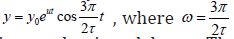 is a frequency of oscillations depending on the time delay τ . Thus, the bigger is a time delay, the lower is frequency of oscillations in a system.
is the imaginary unit. By substitution of the requested solution in the form (9) into the equation (8) the equation for calculation of the Eigen values is got (after deletion by Applying the Euler’s formula for exponents of imaginary numbers, for the real and imaginary parts of this equation yields the following equation array:, , where from follows: at v=0 two processes are possible: monotonously exponentially increasing (u>0) and decreasing (u< 0) in time. Obviously the region by is , n = 0,1,2,.. for u > 0 . Accounting that v is considered positive, from the second equation (6) yields the attainable region by parameter therefore the common region by v is Thus, the oscillating solution growing in time is realized by which means that it starts from vt=3π/2 , when exponentially growing with time solution (9) begins oscillations leading to disintegration of the system. For unstable regime the equation (8) results in is a frequency of oscillations depending on the time delay τ . Thus, the bigger is a time delay, the lower is frequency of oscillations in a system.Critical Levels in the Systems and Optimal Control of the Development
The corresponding critical values of the system achieved during the stable development are estimated as follows:  , where from follows that before starting v ≠ 0 the achieved by v = 0 status of the system is
  The last is solved with
  is estimated as critical level of the parameters. Consequently
  when τ = 0 , and
  for τ ≠ 0 . The higher is time delay, the lower is growing rate of the system and the narrower is region by parameters u , v . Thus, when v ≠ 0 , the oscillating modes of system’s development with exponentially decreasing (u < 0) and exponentially increasing (u > 0) amplitudes become available. In the first case, the oscillating system decays with time and is sustainable (can lead to degeneration of the system, the cessation of its operation), whereas in the second case, growing over time, the oscillation process will quickly destroy the system (growing in time instability cause catastrophe). For example, in a case of financial systems this means that the rocking of growth and decrease leads to a total collapse. So one needs to find the conditions, under which prevention of mode oscillations growing with time is possible (control of the system). Thus, it has to evolve, growing smoothly, without oscillations. From such general speculations one can come to a conclusion, that the financing of the project should be closely monitored for features of the development, which are modeled by the appropriate equations and scheduled for possible delays in time.
, where from follows that before starting v ≠ 0 the achieved by v = 0 status of the system is The last is solved with is estimated as critical level of the parameters. Consequently when τ = 0 , and for τ ≠ 0 . The higher is time delay, the lower is growing rate of the system and the narrower is region by parameters u , v . Thus, when v ≠ 0 , the oscillating modes of system’s development with exponentially decreasing (u < 0) and exponentially increasing (u > 0) amplitudes become available. In the first case, the oscillating system decays with time and is sustainable (can lead to degeneration of the system, the cessation of its operation), whereas in the second case, growing over time, the oscillation process will quickly destroy the system (growing in time instability cause catastrophe). For example, in a case of financial systems this means that the rocking of growth and decrease leads to a total collapse. So one needs to find the conditions, under which prevention of mode oscillations growing with time is possible (control of the system). Thus, it has to evolve, growing smoothly, without oscillations. From such general speculations one can come to a conclusion, that the financing of the project should be closely monitored for features of the development, which are modeled by the appropriate equations and scheduled for possible delays in time.
The control of any CDS has not only to consider the time lag, but it has also to account the forecast, and therefore the mechanism of adjustment of the managed system, its sustainability must be proactive. Therefore, in many cases, the development management of the systems requires simultaneous and consistent taking into account both the time delay and the switching mechanisms of adjustment (adaptation) of the system under the future features. To study characteristic mechanisms of timing and their impact on sustainable development of systems it can be considered, for example, the following mathematical model:

Where τ is the time forecasting term of the system.
Equation (10) means that the rate of development of the system described by the mathematical model, that focuses not on current performance as in equation (1) and not on previous performance as in equation (8), but on a future performance. To solve equation (10), the initial conditions on the time interval from zero to τ must be specified. For example, funded project and its execution at each moment of time have a rate that does not match the current level of funding, and one that meets the future, a higher level, which is the head. This is a case of development in advance. Modeling the development of complex systems with forecasting terms has interesting features that are worth exploring and are used for optimal control of systems’ development (processes).
Considering solution of the equation (10) in the form (9) and substituting the solution sought  the equation to determine the Eigen values (after reduction by ezt ) yields: zτ = kτezt.Researching possible solutions of this equation yields the highest value kτ by which solution exists, under conditions: uτ =1,kτ=1/e where it is clear that as similarly to the equation with a time delay, when v = 0 , there are two cases: exponentially increasing (u > 0) and exponentially decreasing (u < 0) in time. When v ≠ 0 , the oscillating modes of development in a system with exponentially decreasing (u < 0) and exponentially increasing (u > 0) amplitudes take place. In the first case, the process of oscillation is damped over time and is sustainable (can lead to the degeneration of the system, the cessation of its operation). But in the second case, growing over time, the oscillations quickly destroy the system. Only here the conditions above, in a contrast to the case of delay, define the lower boundary of the steady growth of the system. The rates of development of the system, taking into account forecasting in time that are below u = 1/τ , will lead to increasing time-oscillations of the system, leading to its destruction.
the equation to determine the Eigen values (after reduction by ezt ) yields: zτ = kτezt.Researching possible solutions of this equation yields the highest value kτ by which solution exists, under conditions: uτ =1,kτ=1/e where it is clear that as similarly to the equation with a time delay, when v = 0 , there are two cases: exponentially increasing (u > 0) and exponentially decreasing (u < 0) in time. When v ≠ 0 , the oscillating modes of development in a system with exponentially decreasing (u < 0) and exponentially increasing (u > 0) amplitudes take place. In the first case, the process of oscillation is damped over time and is sustainable (can lead to the degeneration of the system, the cessation of its operation). But in the second case, growing over time, the oscillations quickly destroy the system. Only here the conditions above, in a contrast to the case of delay, define the lower boundary of the steady growth of the system. The rates of development of the system, taking into account forecasting in time that are below u = 1/τ , will lead to increasing time-oscillations of the system, leading to its destruction.Strategies for Sustainable Development
The above considered forces to conclude that for sustainable development of the system both processes of the time delay and time forecasting must be correlated in a system development. This can be treated as the global law of optimal control for the CDS. From the expressions obtained for critical levels of delay systems follows that the ratio of the growth rate for the delayed type and forecasting type systems’ development is approximately equal to 1.293. By Zhirmunsky & Kuzmin [11] it is possible to recommend the following method for determining the development of the system and its critical points, illustrating the process according to Figure 5, where the two critical curves are in the first quadrant, respectively, for strategies with a delay (top) and forecasting (bottom). In any case, a stable development is possible only between these two strategies and the actual behavior of the system can be only inside the region between them. Example of building the control strategy for system with prevention of critical regimes in steady development is considered below. Given the peculiarities of the behavior of systems development with shifted arguments, one can construct a control strategy in the following way. Let at the initial moment of time (t = 0) the intensity of development equal to 0 u , delay is absent (τ = 0) , so the system according to (9) develops following the law  until the time t = t1 , where the delay is equal to
  then it must switch the rate of development to the limit, which is leading to the arguments
until the time t = t1 , where the delay is equal to then it must switch the rate of development to the limit, which is leading to the arguments
Next, the system continues stable growth with the new rate u1 point-in-time  when the delay reaches a critical level of development for a strategy with delay (Figure 4). Then again, one can go to the lower critical curve, which corresponds to the development strategy with forecasting, that is
  . And so on to provide the desired level of system development. is clear that over time of the system’s development with growing time delay such control becomes ineffective so that it’s best to stop and then continue the development, starting it again with zero delay.
when the delay reaches a critical level of development for a strategy with delay (Figure 4). Then again, one can go to the lower critical curve, which corresponds to the development strategy with forecasting, that is . And so on to provide the desired level of system development. is clear that over time of the system’s development with growing time delay such control becomes ineffective so that it’s best to stop and then continue the development, starting it again with zero delay.The Method of the Dynamics of Average
The Markov chains can be used in the description of different engineering, economic, ecological problems and many other CBS. Based on the initial description of the problem, when the states of the system are determined and their interconnections are known, the application of the Kolmogorov theorem for probabilities of the dynamic states of the system allows following all the evolution of it [27]. In practice, more popular is the method of the dynamics of average, which is obtained from the Kolmogorov theorem for the closed system with its averaging by probabilities of the states at each moment of time. We may use graphs for the system with discrete states. The vertices of the graph correspond to the states of the system in Figure 6. The arrows between graphs show the possibility of system’s transfer from one state to another one.
This way a very complex system may be easily modeled because there is the mnemonic rule for the differential equations written for each system after all the initial conditions, states, and their interconnections are stated. Here i m is an average amount of a matter under modeling, and ij λ are intensities of the transformations from the state with index i to the state with index j . The standard equation array of the dynamics of average is got as follows. In the left part of each equation there is a derivative of the average value (expected value of the i -th state), and in the righthand side there is the sum of the products of the probabilities of all states from which arrows lead to a given state, by the intensity of the corresponding event streams, minus the total intensity of all streams that deduce the system from the given state. For example in case of Figure 6 it is:

The system (11) can be illustrated in the following way. Let’s consider a system of failure type of a certain kind of products and their repair and restoration, which can also be similarly extended to other cases, which are described by similar equations. Let us have N products, which gradually fail with the intensity 12 λ per unit time, but restored on average with intensity 21 λ . Then the graph of states shown in Figure 6 for this stochastic system represents 1 m and 2 m as the average quantities of given matter in the states 1 and 2, respectively. One can imagine that this way the very complex big systems can be described and modeled on the computer because such standard equation array of the sordinary differential equations is easily solved numerically. For example, automated system for factory or robotics (separate robot with the interaction of its elements or common operation of interacting robots) may be modeled.
The initial condition for equation array (11) is stated as

With the condition of the closed probability system, the sum of all probabilities of all states is equal to unity for each moment of time. This means for our average values that the amount of regular and defective products is always constant and equal to the initial whole quantity of the products in a system: 1 2 m + m = N . Proceeding from the latter, the solution of the system (11) can be considered by choosing any of the equations, after which the second equation has to be identical. The following one of the possible solutions satisfies the initial conditions (12):

Generalization of the Method of the Dynamics of Average for the Systems with Shifted Arguments
The solution (13) shows a gradual decrease over time of the number of regular tools with any ratio of the intensity of failure and repair of the tools (return to the state of service). Consider this task, taking into account the influence of shifted (deviating) arguments. For example, a return of the repaired products may occur for certain reasons with the certain delays (or similarly - their receipt for repairs) or the company is guided by a certain advance of the products coming for repair. So, in the first case:

A delay starts its influence from the moment t ≥τ . In a second case correspondingly:

In a case of both time delays and time forecasting it follows:

The delay starts acting here from the moment of time 2 t ≥τ . Advance is equal 1 τ .
First consider the system (14) seeking the solution in a form:

Put (17) into (14), and one can get the characteristic equation as follows

Then substitute the complex characteristic value z = u + iυ into(18) and get the system of two equations for the real and imaginary parts, respectively:

The equations(19) show that the unstable regimes are absent because υ ≠ 0 is got by the division of the first equation on the second one:

It is seen from the second equation (20) that a function u can be only negative due to positive term in the brackets by u ≤ 0 . By positive u , the expression in the brackets is always positive, and (20) gets in contradiction as far as the right side of the equation (20) can be only negative value. Thus, the process can be oscillating but the system remains always stable. And a solution has the form

The obtained (21) shows that an amount of the regular functioning tools (or repaired, returned to the functioning state) is going with a running of time to its asymptotic boundary  where 12 21 α =λ12/λ21 is. Consecutively, a system is aiming to its constant value determined by a ratio of intensities of the failed and repaired tools.
where 12 21 α =λ12/λ21 is. Consecutively, a system is aiming to its constant value determined by a ratio of intensities of the failed and repaired tools.
Similarly, we can consider the other cases, for example, the following ones. For example, an analysis of solution obtained for the model with advance arguments (15) leads to a conclusion that a system with an advance shift in time can advantage the system’s development but it can also cause instability of a system, which is a strong disadvantage because it can lead to a system’s disintegration.
The Methods Applied
We applied in our investigations the analytical and numerical methods for the solution of the differential and integro-differential equation arrays modeling the CDS, for the linear, as well as for the non-linear tasks. Now in a lot of CDS of diverse nature, the hereditary processes are modeled so that the fractal theory and generalized fractional integro-differential calculus is considered as most appropriate.
Discussion
The examples considered in this paper represent the analytical and numerical study of the linear and nonlinear simple differential equations and complex equation arrays. Starting from the simplest linear development equation (1) first considered by T.R. Malthus, who got exponential growth of system with a constantlygrowth rate, we have shown how much solutions of the same equation (8) with just time delay may differ from the one by Malthus. The time delay is coming naturally as far as many systems have hereditary properties (alive and technical ones) when their state at the current moment depends not only on parameters of the system in this moment of time but also on some history of the system’s development. In this case, exponential growth is available of two types: stable and unstable. What is more, there are critical levels in a development, which are got time to time during the system’s development. And the optimal stable strategy is the piecewise non-continuous, with a growing rate switched all the time in the critical points.
The simplest nonlinear equation (7) reveals stable monotonous development till the top boundary. Such kind nonlinear equations with time delays do not reveal any instability in contrast to the linear one, so that monotonous character is supplied by restriction term (like the limited resources or other kind restrictions dumping instabilities). These phenomena were demonstrated too on the CDS described by the equation array containing a lot of parameters (in our case 6 equations, which have a lot of different time delays by different parameters of the system). The restrictions for the growing parameters from the top stabilize the system in a complex case as well.
The last example has a concern to the application of the simple method of the dynamics of average, which is based on the Kolmogorov theorem for the Markov processes. It was shown the generalization of the method for the systems with shifted arguments. It may give the new highly productive life of this method due to its simple realization, especially with the application of computer simulations and for big and very big systems (thousands and even millions of the states!). The simplicity of this method is due to the possibility of usage of the mnemonic rule for the formulation of the differential equations based on the given description of all states of the CDS and intensities of their interactions. The last ones mean that only description of the CDS is needed, for example in a form of the graph with intensities of the states’ connections. All the other is done on the computer.
Conclusion and Future Research
The example of the PHO’s model developed by us was demonstrated available for computer simulations to reveal the features of the nonlinear CDS’ functioning. Surprisingly, it was shown that nonlinear systems with limitation by development for each of their parameters are stable, in a contrast to the linear systems with time shifts, which are prone to instability by some parameters. It was clearly shown in the numerical computation for the system of 6 equations and analytically for one nonlinear equation solved.
The method of the dynamics of average was adopted for an application to the analysis of the CDS with deviated arguments. For the simple case of two states, an analytical solution for the CDS with delay and advance in time was shown. The method may be further developed in a lot of diverse applications as far as it is simple in realization for any big systems.
To Know More About Robotics & Automation Engineering Journal Please click on: https://juniperpublishers.com/raej/index.php
No comments:
Post a Comment